|
|
|
|
|
CONTENTS |
|
|
|
|
|
Introduction |
|
4.1.1.
|
The mass - friction interaction model. |
|
4.1.2. |
Tidal
forces acting upon the lithosphere. |
|
4.1.3.
|
Generation of Earth Tide Values. |
|
4.1.4.
|
Seismicity compared to one year’s period Earth-tide
wave. |
|
4.1.5.
|
Seismicity compared to 14 days period lithospheric
oscillation. |
|
4.1.6. |
Daily
Earth-tide oscillation, correlated to same day seismicity (29/05/2001). |
|
4.1.7.
|
Examples of “a posteriori” correlation of Earth-tide
waves to seismicity. |
|
4.1.8.
|
Statistical test of seismicity to 14 days tidal
oscillation. |
|
4.1.9.
|
Statistical test of seismicity to daily tidal
oscillation. |
|
4.1.10.
|
Electrical signals timing, compared, to lithospheric
tidal oscillations. |
|
|
a.
SES, (Seismic Electric Signals) or “high frequency”
signals. |
|
|
SES generated by the
Izmit, EQ (17/8/1999, M=7.5), in Turkey . |
|
|
SES signals recorded by
HIO monitoring site, compared to 14 days period tidal lithospheric
oscillation. |
|
|
SES signals recorded
by PYR monitoring site, compared to 14 days period tidal ithospheric
oscillation. |
|
|
SES signals recorded
by ATH monitoring site, compared to 14 days period tidal lithospheric
oscillation. |
|
|
b.
Oscillatory type earthquake precursory signals. |
|
|
c.
VLP signals. |
|
|
|
|
|
 |
|
4.1. Time of EQ occurrence
determination.
Introduction
After a strong earthquake has occurred at a seismogenic area, the
immediate question which arises, is: when will it strike again? The
seismologists worked out this question firstly because of its
societal significance. This question implies, although in an
indirect way, that the seismogenic area is already known and the,
expected, magnitude of the future earthquake is almost similar, in
magnitude, to the previous one or strong enough, so that it must be
taken into account, seriously.
At the early steps of the scientific research for a successful
earthquake prediction, the recurrence times of strong earthquakes,
at a specific seismogenic area, were analyzed with statistical
methods. The obtained, results refer to the long-term prediction,
mainly. The fact that strong earthquakes are not very frequent
prohibits, increased time resolution of the statistical methods
which are used, due to the fact that the “sampling interval” is too
long. A different statistical scheme, analyzes the frequency –
magnitude dependence and their logarithmic proportionality, the
“b-value” (Ma 1978, Smith 1986, Molchan et al. 1990) and variations
of coda Q (Jin and Aki 1986, Sato 1986). Major earthquakes have been
preceded by seismic quiescence. Kanamori (1981), Lay et al. (1982)
Wyss et al. (1988) reviewed the methodology. Scholz (1988) studied
the mechanisms, which could be responsible for this phenomenon,
while Schreider (1990) proposed a statistical basis for making
reliable predictions, based on quiescence. Gupta (2001) used the
same methodology for the medium-term forecast of the 1988 northeast
India earthquake.
As a result of this inability of the statistical methodologies to
provide adequate time resolution (predictive time window for the
future strong earthquake), which could be of some use for the
society, different methodologies, more sophisticated, were developed.
The algorithm CN is one of them (Keilis-Borok et al. 1990). This
algorithm allows diagnosis of the times of increased probability of
strong earthquakes (TIPs). The CN stands for the application of the
TIPs methodology for California – Nevada, while a version addressed
to magnitudes larger than M=8R is assigned the name “algorithm M8” (Keilis-Borok
and Kossobokov 1990; Romachkova et al. 1998).
Varnes (1989) studied the accelerating release of seismic energy or
seismic moment either to time elapsed, or to time remaining, in the
period preceding a main shock. He introduced empirical relations,
having origins in both experiment and physical theory, going back
many decades. The acceleration process was analyzed in laboratory
experiments and was applied before strong earthquakes in Kamchatka
and Italy by Di Giovambattista and Tyupkin (2001).
Narkunskaya and Shnirman (1990) proposed the multiscale model of
defect development. Following this methodology and through
simulation of the lithosphere, to a hierarchical discrete structure,
which consists of some singularities, allows one to predict the time
of appearance of “large” defects.
According to the Load-Unload Response Ration (LURR) methodology,
when a system is stable, its response to loading corresponds to its
response to unloading, whereas when the system approaches an
unstable state, the response to loading and unloading becomes quite
different (Yin et al. 1995, 1996, 2002).
Seismic quiescence and accelerating seismic energy release can be
further detailed by the use of the RTL algorithm. This algorithm (Sobolev
2001, Sobolev et al. 2002, Di Giovambatista et al. 2004) analyze the
RTL (Region, Time, Length) prognostic parameter, which is designed
in such a way, to have a negative value if, in comparison with long-term
background, there is a deficiency of events in the time – space
vicinity of the tested area. The RTL parameter increases if
activation of seismicity, takes place.
Seismicity “Pattern recognition algorithms” such as “ROC” – range
of correlation – and “Accord” were used by Keilis-Borok (2002) to
identify premonitory patterns of seismicity, months before strong
earthquakes in Southern California. Another version of the pattern
recognition methodology takes into account the earthquake
intensities, in order to forecast the time of occurrence (Holliday
et al. 2006).
In the RTP (reverse tracing of precursors) methodology, the
precursors are considered in reverse order of their appearance (Keilis-Borok
et al. 2004).
The methodology of “Space-time ETAS” (Ogata et al. 2006) is a
further extension and improvement of the seismic quiescence
methodology. ETAS stand for Epidemic Type Aftershock Sequence.
Yamashina (2006) used the statistical test of time shift for
prediction studies in Japan.
The algorithm SSE (subsequent strong earthquake) was designed for
prediction of relatively strong earthquakes following a strong
earthquake. A subsequent, strong earthquake can be an aftershock or
a main shock of larger magnitude.
The SSE algorithm resulted from the analysis of 21 case histories
in California and Nevada. Then, it was, retrospectively, tested in 8
seismic regions of the world (Gvishiani et al. 1980, Levshina et al.
1992, Vorobieva et al. 1993, Vorobieva et al. 1994, Vorobieva 1994,
Vorobieva 1999).
The statistical treatment of the earthquakes, which occurred at a
specific seismogenic area in the past, has been proved more or less
sufficient for the “medium-term or long-term” earthquake prediction.
In terms of the “sort-term” prediction the seismological literature
has, not even a successful case, to present at all. Apart from the
long time sampling interval, which elapses between two consecutive
strong earthquakes in the same seismogenic area, there is an
intrinsic difficulty in using statistical methods towards a
successful, sort-term earthquake prediction. This is analyzed as
follows.

4.1.1. The mass - friction interaction model.
Any seismic event can be simulated by the following model,
presented, in figure (4.1.1.1), and introduced, by Shimazaki and
Nagata (1980). A mass, standing on the surface of a media, is pulled
by a spring. As long as the pulling force (e), which is applied on
the mass through the spring, is less than friction (τ) that exists
between the mass and the media surface, the mass does not move.
Consequently, each time there is inequality between friction and the
pulling force (e) that is:
τ <= e
(4.1.1.1.)
then, the mass starts moving and therefore due to the fact that the
spring becomes shorter, the previous equation turns into the
inequality:
τ > e
(4.1.1.2)
This is graphically, presented, in the following figure (4.1.1.1).

Fig. 4.1.1.1. The
spring (mass-friction) model introduced, by Shimazaki
and Nakata (1980).
A seismogenic area behaves in a similar way and in a first
approximation. The seismogenic area is stress-strain, charged, for a
time period (fig. 4.1.1.1a), until it reaches the critical,
fracturing, stress-strain level. At this time, an earthquake (EQ)
takes place and the overall, stress-strain load discharges (at Δτ)
to a lower level. If we assume that the critical, fracturing level
and the discharge level are constant, then the recurrence time
period of a strong EQ is determined by the time interval which
elapsed between two consecutive EQs. This mode of recurrence time
periods is called “strictly periodic”. This mode of charge –
discharge procedure of a seismogenic area is just a theoretical
approximation and does not reflect what is observed in nature.
Next model (fig. 4.1.1.1.b) assumes that the stress-strain charge
is released through EQs of variable magnitudes (time predictable) to
different final lower levels.
As an immediate result of this mode of energy release in a
seismogenic area, different recurrence EQs times are observed. This
is very common in the seismic activity, observed, in a specific
seismogenic area. Consequently, a strong difficulty is imposed on
any statistical analysis of the recurrence times of these EQs.
A third adopted model (slip predictable), is the one, presented, in
figure (4.1.1.1c). In this case, the fracturing, stress-strain level
is variable, while the lower, stress-strain discharge level is
accepted as constant. Also, this model justifies the variable
recurrence times of earthquakes in the same seismogenic region and
implies the very same difficulties in the statistical determination
of the recurrence time of these EQs.
Both models, “time predictable” and “slip predictable”, suggest the
inability to apply statistical tests for the short-term prediction.
Moreover, it is not yet clear in nature which model is valid, each
time a strong EQ is pending in a seismogenic region. Therefore, a
more generalized model is postulated, in which both the
“stress-strain” fracturing level, as well as the lower “discharge
level”, are considered variable. This model is presented in the
following figure (4.1.1.2).

Fig. 4.1.1.2. A more generalized model of a seismogenic area in
which both the “stress-strain” fracturing level, as well as the
lower “discharge level”, are considered variable.
The introduction of variability in both, the stress-strain
fracturing level as well as to the lower discharge level complicates
much more the problem of studying the recurrence time of strong EQs.
Finally, the small magnitude random seismicity, which takes place
in the time period which elapses in between two strong earthquakes,
modifies the overall time T which is expected to elapse between them
(Hori and Oike, 1999). This is explained by the following figure
(4.1.1.3).
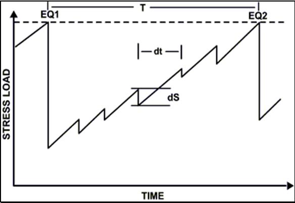
Fig. 4.1.1.3. Modification of time T, elapsed, between EQ1
and EQ2, due to small size seismicity which occurred in the same period of
time in a specific seismogenic area, due to its small size
seismicity (Hori and Oike, 1999).
What is interesting, in this mechanism, is the fact that, each time
when a small earthquake occurs, the seismogenic area is, slightly (dS),
stress-strain, discharged and therefore, it takes some time:
Δt = dS / (dS/dt).
(4.1.1.3)
Where:
Δt is the time, needed, by the seismogenic area, in order to
recover to its previous charge state.
dS is the temporary stress-strain discharge, due to small size
seismicity
dS/dT is the rate of stress-strain change of the seismogenic area,
during this time period to recharge up to the previous state of
stress – strain level.
Consequently, the overall time period T, between two consecutive,
strong earthquakes, depends on the small size seismicity of the
seismogenic area itself, too.
So far, all these models suggest a chaotic behavior of the
seismogenic area, in terms of the time of occurrence of a strong EQ.
This chaotic behavior of the seismogenic area, justifies what the
seismologists accept as inability to predict a strong EQ in
“short-term time”.
This unsolvable problem can be formulated, as follows, in a simple
mathematical approach:
Let us assume that, before a strong EQ, the stress-strain charge of
the seismogenic area is represented by a linear function:
S = at + b
(4.1.1.4)
Where (S) is the total stress-strain charge at a time (t), (a)
represents the value dS/dt, (b) is a constant, while (Sfr) is the
fracturing level (fig.4.1.1.4).

Fig. 4.1.1.4. The adopted, simplified model indicates the
mathematical relation of the stress-strain charge, as a
function of time, to the fracturing level of the seismogenic area.
Following these annotations, an earthquake occurs when at a certain
time (t) both equa-tions:
S = at + b and S = Sfr
(4.1.1.5)
are satisfied.
In the case of equations (4.1.1.4), the parameters (a), (b) and (Sfr)
for a seismogenic area and for a certain time period (T), are
unknown. Therefore, the time (t0) for the occurrence of a strong EQ
can be determined, only, after having assigned arbitrary values on
the parameters of equations, present in (4.1.1.5). In mathematical
terms, this suggests that the system of equations (4.1.1.5) is
undefined and therefore, there is an infinite number of solutions,
referring to (t0), the time of occurrence of the future, strong EQ.
The space of solutions of equations (4.1.1.5) incorporates a)
arbitrary solutions in (t0), which have no seismological
significance (in terms of stress-strain charge status of the
seismogenic region) and b) true solutions in (t0), which are closely
related to the real strong earthquakes which will take place at the
(t0) time in the future. Therefore, the real “time prediction
problem” is to find a way to distinguish the (b) type solutions of
equations (4.1.1.5), from the infinite space of its arbitrary
solutions.
The statistical schemes, which are used to date, have been proved
unsuccessful to this end. In contrast to the used statistics, the
solutions of equations (4.1.1.5) will be constrained by the use of a
specific physical model, namely “the lithospheric oscillating plate”,
which was presented in section (2.5.2). In practice, the “AND”
operator of the Boolean algebra, is used between the solutions of
the equations (4.1.1.5) and the solutions which result from the use
of the lithospheric, oscillating plate model.
The stress charge in the future EQ focal area is due to two stress-increasing
mechanisms:
The first one is the plate’s motion. The
motion of the local lithospheric plates is the most important factor
in stress increase in a specific seismic area. The following figure
(4.1.1.5) presents the tectonic plate’s model, which holds for the
Aegean area, Greece (McKenzie 1972, 1978).

Fig. 4.1.1.5. The Aegean area, plate models proposed, by
McKenzie (a - 1972, b - 1978).
The kinematics of the same area was studied by Papazachos et al.
(1996). The active, crustal deformation in the Aegean and the
surrounding area appear in the following figure (4.1.1.6).
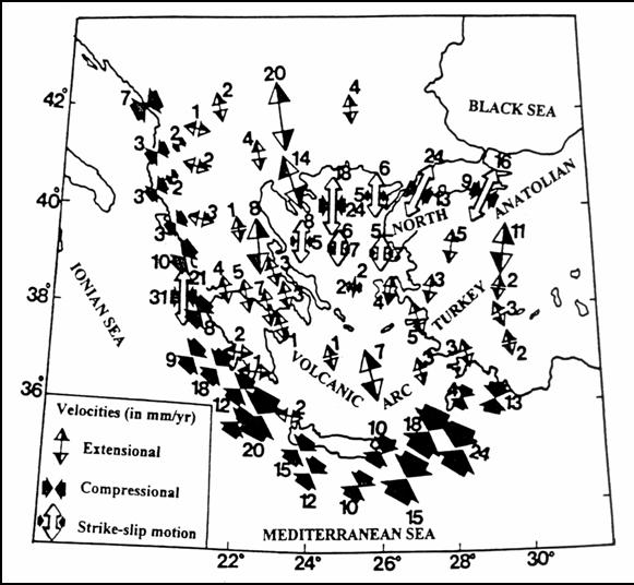
Fig. 4.1.1.6. Plate kinematics and crustal deformation in the Aegean
area (after Papazachos et al., 1996)
The second is the lithospheric
plate oscillation, as it was briefly presented in section (2.5.2).
The influence of the tidal forces upon the Earth’ surface and their
effect, as a triggering mechanism upon the generation of earthquakes,
had been also studied by Tamrazyan (1967, 1968), Liu et al. (1985),
Shirley (1988), Bragin et al. (1999), Thanassoulas et al. (2001a,
b), Duma et al. (2003), Tanaka et al. (2006).
In this section, a more detailed analysis will be presented, as far
as it concerns the way the tidal forces affect the stress-strain
charge status of a seismogenic area which is considered as subjected
to tidal forces (T).
4.1.2 Tidal forces acting upon the lithosphere.
The tidal forces (T) which are applied on the lithosphere (fig.
4.1.2.1) are decomposed in to two components: a) the horizontal (Tx),
and b) the normal (Tz), to the lithosperic plate.

Fig. 4.1.2.1. Analysis of the tidal force (T) into its
horizontal (Tx)
and vertical (Tz) components.
Furthermore, the (Tx) component can be analyzed into its horizontal
subcomponents, related, to the strike of the existing fault in the
seismogenic area. Therefore, assuming that:
Tv = Tx
(4.1.2.1)
The orthogonal analysis of (Tv) into two axes, one normal to the
fault strike and the other along it, results into the horizontal
tidal forces components of Tal (along the fault strike) and Tnm (normal
to fault strike), presented, in the following figure (4.1.2.2).

Fig. 4.1.2.2. Analysis of the horizontal (Tv) component of the tidal
force, into two orthogonal components (Tal, Tnm), along and normal
to the seismogenic fault strike.
The horizontal tidal component (Tv) is the same (in amplitude and
direction), in both sides of the seismogenic fault. Consequently, no
stress-strain increase or decrease can develop in the fault zone
which in turn will modify its overall stress-strain charge.
On the contrary to the horizontal component, the normal one (Tz) to
the lithospheric plate will force it to oscillate in the same
frequency spectrum, as the tidal forces oscillate. A sketch drawing
of the oscillating lithospheric plate is presented in fig.
(4.1.2.3).

Fig. 4.1.2.3. The lithospheric plate oscillates, triggered by the
oscillating tidal forces. The dotted rectangle is the lithosphere at
its rest position, while the solid, curved rectangle represents the
oscillating lithosphere. Double arrow indicates the oscillation
amplitude.
The lithospheric oscillation has a significant consequence. The
length of the part of the lithospheric plate that oscillates,
changes, due to its oscillatory deformation. This is presented in
the following figure (4.1.2.4).

Fig. 4.1.2.4. Change of length L0 of lithosphere in to L1, due to
its oscillation.
Moreover, the oscillating lithospheric plate increases its distance
from the Earth’s center at (dR), where (R) is the radius of the
Earth at the seismogenic area. By denoting as (φ) the angle, which
is defined by the oscillating lithospheric plate (arc) and the
center of the Earth (fig. 4.1.2.5), then the following equation
holds:
dL = φ . dR
(4.1.2.2)

Fig. 4.1.2.5. Sketch drawing that indicates the deforming
mechanism of the oscillating lithospheric plate.
By taking into account that (dR) is an oscillating parameter, due
to tidal forces and the strain definition (Jaeger, 1974) of (ε) as:
ε = dL/L
(4.1.2.3)
and by combining (4.1.1.2) with (4.1.2.3), it results into an
oscillatory strain (ε) component, with its maximum effect, applied,
at the center of the plate. Therefore, for a monochromatic
lithospheric oscillation, the strain will have the form:
ε = ε0 . sin (2πΤ-1t)
(4.1.2.4)
where: (Τ) is the period of oscillation.
The oscillatory strain, represented by equation (4.1.2.4),
generates the corresponding compressional and extensional forces S (fig.
4.1.2.6), required, to trigger an earthquake, in any fault that is
close to rapture.

Fig. 4.1.2.6. Compressional and extensional oscillatory forces (S),
generated, in the lithosphere, due to its tidal oscillation.
Furthermore, the oscillating lithosphere is charged with energy,
due to its deformation as follows:
W = ½ (σ1ε1+ σ2ε2+ σ3ε3)
(4.1.2.5)
Where (W) is the potential energy per unit volume, or strain energy
per unit volume, (σ1, σ2, σ3), are the principal stresses and (ε1,
ε2, ε3) are the principal strains.
In conclusion, a seismogenic area is charged with a slow, in time,
linearly increasing strain, due to the motion of the lithospheric
plates and simultaneously, its strain charge oscillates due to tidal
forces.
In section (2.5.2), it was pointed out that, an earthquake would
occur when the, combined, linearly increasing and oscillating stress
reaches the fracture level of the seismogenic area. Moreover, in
section (4.1.2), was presented the importance of the normal to the
lithosphere force, which triggers its oscillation, and concerns, its
effect on the lithospheric, stress-strain charge. Consequently, it
is of great interest to know, in advance, the way the vertical
component of the Earth tide evolves in time, since this is the
driving mechanism of the lithospheric, tidal oscillation. The tidal
peak values, generated, from the combination of the various Earth
tidal components, are the most probable times of occurrence of
strong earthquakes (fig. 2.5.2.9).
4.1.3 Generation of Earth Tide Values.
Many scientists have presented Earth-tides generation procedures,
in the scientific literature. Some of them are: Doodson (1928),
presented an analysis of tidal observations, Pertsev (1958),
presented an harmonic analysis of the Earth-tides, Munk et al.
(1966), analyzed the frequency spectrum of Earth-tides, Godin
(1972), presented an analysis, too, Schuller (1977), used the hybrid
least squares frequency domain convolution method in tidal analysis,
Rudman et al. (1977), presented a FORTRAN algorithm for the Earth-tide
gravity data generation, De Meyer (1982), used a multi input –
single output model for the Earth-tide data, Melchior (1983),
presented a monograph on Earth-tides, Tamura (1987), calculated the
tide generating potential by harmonic analysis, Tamura et al.
(1991), used a Bayesian information criterion for tidal analysis,
Wenzel (1994), presented the package ETERNA for tidal data analysis,
Venedikov et al. (1997), presented a software package for tidal data
processing, Venedikov et al. (2000, 2001), calculated the Earth-tide
constituents of degree 3 and 4, by using superconductive gravimeters,
Venedikov et al. (2003), presented the VAV package for tidal data
processing.
Rudman’s et al. (1977) methodology addressed, directly, the problem
of tidal effects on the gravity measurements in any gravity project.
In principle, this methodology corrects the gravity measurement
taken, at any place, for the elevation difference which is caused by
the tidal waves. This gravity correction is directly, correlated, to
the stress-strain oscillating mode of the lithosphere, due to its
tidal oscillation. Therefore, graphs of the oscillating gravity
corrections (in mgal), generated, for a specific place, indicate,
indirectly, its strain-stress oscillating, lithospheric mode. In
mathematical terms, it is expressed as:
S = kTc
(4.1.3.1)
Where: S is the oscillating stress-strain component of the
seismogenic area
Tc is the tidal gravity correction, calculated, by Rudman’s method
K is a constant, which transforms Tc into S
The methodology, used, by Rudman et al. (1977), is based on the
equations which derived by Garland (1965) and Bartels (1957).
Vertical derivatives of these potential functions yield the desired
components of gravity, in terms of Legendre Polynomials. The
implementation of the computer package was based on the work of
Goguel (1954) and Longman (1959). Geophysicists used, extensively,
this methodology and also, the published, by the European
Association of Exploration Geophysicists (EAEG) tables, to apply
tidal corrections in gravity surveys, which are dated back for many
years.
Samples of tidal gravity correction values have been calculated
with Rudma’s method for a time period of (2) days, with sampling
period of one (1) minute and are presented in the following figure
(4.1.3.1).

Fig. 4.1.3.1. Gravity correction tidal data was generated by
the Rudman’s et al. (1977) method, for the period 14-15 February 2007.
The dashed, vertical lines indicate hour time period, the red,
dashed lines indicate start of the day, and the solid, black line
represents the tidal data in mgals.
The 24-hour period oscillation of the Earth’s tide is clearly
presented, as the 12 hours period is, as well. If we consider a much
longer time period of tidal data, it is possible to filter out
periods of a day or less and to visualize oscillations of much more
longer periods. This task is performed, simply, by applying
Shannon’s sampling theorem. If a data series is sampled by a
sampling interval of Δτ, then the lowest period which is preserved
in the sampled data set, is 2Δτ (Nyquist period). The entire
operation behaves as a low-pass filter.
In the previous case (of longer data set), we apply a sampling
interval of one (1) day. Therefore, daily tidal oscillations will be
filtered out, since the maximum period, preserved, in the sampled
data, is two (2) days. The result of such an operation is
demonstrated in the following figures (4.1.3.2 – 4.1.3.3).

Fig. 4.1.3.2. A three-months period (December 2006 –
February 2007) of tidal data set, sampled at one-minute
interval, is presented.
The result of the application of the re-sampling operation, at a
day’s sample period, on the tidal data of figure (4.1.3.2) is the
data set presented, in the next figure (4.1.3.3).

Fig. 4.1.3.3. A three-month period (December 2006 – February 2007)
of tidal data set, re-sampled at one-day interval, is presented. The
tidal oscillation resembles the M1, Moon declination component.
Next, it is considered a much longer period of four (4) years, with
a day’s sampling interval (fig. 4.1.3.4). In this case, are observed
two distinct tidal oscillations. The first one which is of the
longest period corresponds to the yearly component of the tidal
gravity variations. On top of it is the 14 days period oscillation
of the previous figure (4.1.3.3).

Fig. 4.1.3.4. Four years period (2004 – 2007) of tidal
gravity data (sampled at one day) are presented. The
yearly component is superimposed by the 14 days period
tidal oscillation.
The graphs of figures (4.1.3.2 - 4.1.3.4) have been calculated for
the following geographical parameters:
Latitude : 380, 0’, 0’’ (Athens location)
Longitude : 240, 0’, 0’’ ,,
Height : 0m a.s.l
Time zone : 0
So far, specific peaks of tidal oscillation have been identified.
Starting from yearly period, these peaks span down to 12-hour
periods. Following the analysis which was presented earlier in
section (4.1.2), these peaks correspond to stress-strain peaks of
the seismogenic area, which is affected by the tidal waves.
Therefore, the seismicity which is induced, by the lithospheric
oscillation, must coincide with the corresponding, tidal peaks. This
will be investigated as follows:
4.1.4. Seismicity compared to one year’s period Earth-tide
wave.
The longest period which has been identified so far in the tidal
data, is a year’s period. Following the previous analysis, this type
of lithospheric oscillation strain-stress charge must be mirrored
into the seismicity of a seismogenic region for the same period of
time. To this purpose, the seismic events, per 10 days period of
time, are correlated to the corresponding lithospheric plate
oscillation for a period of a year (2000). The entire Greek
territory is considered as a seismogenic area. This is presented in
the following figure (4.1.4.1). The yearly period Earth tide wave is
presented in the upper graph, while the “per 10 days seismic events”,
are shown in the lower graph.
It is evident that the seismicity increases and correlates well
with the increase of the amplitude of the yearly, tidal wave.

Fig. 4.1.4.1. Yearly Earth-tide wave compared with the seismicity
for the same period of time.
These results strongly suggest the dependence of seismicity of a
seismogenic area to Earth-tide waves, as a triggering mechanism, as
has already been pointed out by earlier papers. In terms of time
prediction it suggests that the predictive time window can be of the
order of a few months, by assuming that a strong earthquake will
occur within this year’s period of time.
4.1.5. Seismicity compared to 14 days period
lithospheric oscillation.
If we consider shorter wavelengths of the lithospheric plate tidal
oscillation, then more interesting results are found. In next figure
(4.1.5.1), is demonstrated the dependence of seismicity to the T=14
days oscillation of the Earth-tide for the period 17/04/2001 –
11/05/2001.
At the same period of the time
only one (Ms = 5.4R, 01/05/2001) strong earthquake occurred. This
seismic event occurred very close to the negative peak of the tidal
oscillation amplitude, following the already, presented, theoretical
analysis.
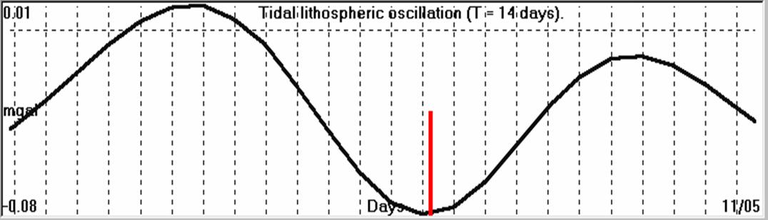
Fig. 4.1.5.1. Seismicity compared to 14-day Earth-tide oscillation
for the time period 17/4 – 11/5/2001. The red bar indicates the
occurrence of the earthquake (M = 5.4R).
The strongest and only one seismic event, EQ (5.4R), occurred on
top of the minimum peak of the tidal wave in this period of time.
4.1.6. Daily Earth-tide oscillation, correlated, to
same day seismicity (29/05/2001).
The same mechanism holds for the day when a strong EQ occurs. The
final extra stress load which is necessary to trigger a strong EQ is
provided by the day’s oscillation of the Earth-tide. Therefore, the
EQ will, most probably, occur at one of the four tidal peaks which
exist in a day’s tidal oscillation (Thanassoulas et al. 2001). The
EQ of the figure (4.1.5.1) is compared with the Earth-tide variation
of the day of its occurrence (fig. 4.1.6.1).
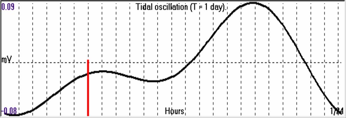
Fig. 4.1.6.1. EQ occurrence time compared with the Earth-tide
variation of the day of its occurrence.
The same EQ, in figure (4.1.6.1), coincides very well with the
first maximum of the Earth’s daily tidal wave (12hour period
oscillation) in its day of occurrence span.
4.1.7. Examples of “a posteriori” correlation of
Earth-tide waves to seismicity.
Since the tidal waves excite the lithosphere in an oscillatory mode,
the triggered, seismicity must correlate to the most basic
frequencies of tidal waves. This is demonstrated as follows.
The seismicity for the period 1995 – 2001 and for seismic events
stronger than 5.5R for the Aegean area is compared with the yearly
period tidal waves (fig. 4.1.7.1).
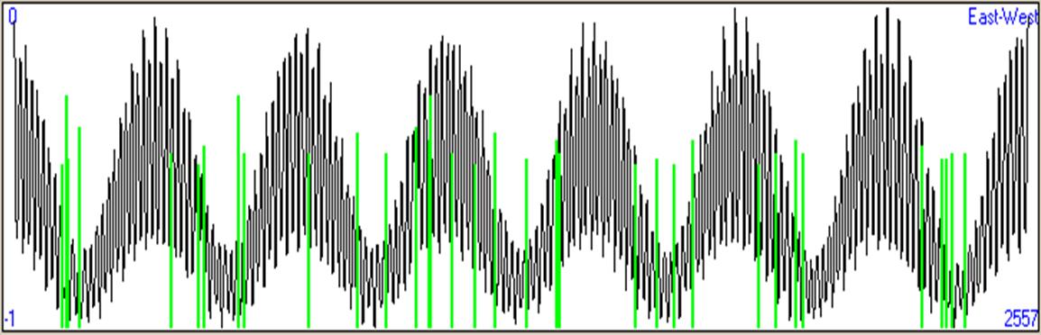
Fig. 4.1.7.1. Yearly tidal oscillation, for the period 1995
– 2001, compared to seismicity (green bars) of the same period.
The seismic events, as a general observation, are clustered at the
“lows” of the oscillation (mainly during June-July), while some
exceptional seismicity exists during years 1997-1998.
The same correlation, between tidal waves and seismicity, holds for
the 14 days period oscillation. This is demonstrated in figure
(4.1.7.2).
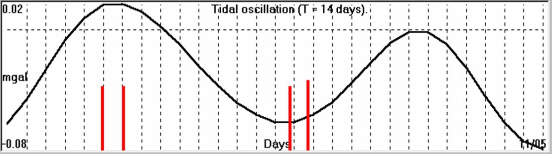
Fig. 4.1.7.2. 14 days period oscillation, for the period
13/04/2000 – 10/05/2000, compared with the seismicity (red bars, Ms>5.0R) of
the same period.
The two double, corresponding seismic events occurred during the
low and high peak of the tidal oscillation.
Finally, the correlation of the time when a strong EQ occurred, to
the daily tidal oscillation, is presented (Thanassoulas et al.
2001), in the following fig. (4.1.7.3).

Fig. 4.1.7.3. Daily, tidal variation, compared to the time
when a strong EQ occurred. The red arrow indicates the EQ time of
occurrence. The time difference between the tidal peak and the time
of occurrence is only 16 minutes.
It is evident, that strong EQs, do not occur at random times, but
they follow, quite well, the amplitude peaks of the tidal wave
oscillation, and follow the triggering mechanism, presented in
figure (2.5.2.9)
4.1.8. Statistical test of seismicity to 14days
period tidal oscillation.
In order to verify the validity of the tidal oscillations to the
seismicity of a seismogenic area, a study has been performed on
strong EQs (Ms>5.5) for the period 1995 – 2001, which are initially,
compared, to the 14 days period tidal wave. The total number of the
seismic events which are studied is forty (40).
The “by chance” percentage (Pch) of the estimation of the correct
day of the occurrence of a strong EQ is:
Pch = 14.28% for a half period (7 days).
In the following table (1) are presented the EQs which were used in
this study. The first column indicates the time in the format
yyyymmddhhmm, the next two are the geographical coordinates, while
the next two are the depth of an EQ in Km and its magnitude in ML, (Ms
= ML+0.5).

The statistical analysis of the data of table
(1), compared, with the corresponding 14 days period tidal
oscillation, gave the following results:
Mean value of time difference of the time of occurrence of the EQs,
from the corres-ponding tidal peak values, for the entire data set,
equals to 1.18 days.
dt Mean Value = 1.18 days
S. Dev. Of dt = 1.15 days
Percentage of EQs with dt = 0 days equals to 39.47% (exact
day)
Percentage of EQs with dt = 0 - 1 days equals to 50.00%
Percentage of EQs with dt = 0 - 2 days equals to 78.95%
Percentage of EQs with dt = 0 - 3 days equals to 100.00
%
A direct comparison of the “by chance” Pch value (14.28%) to the
percentage (39.47%) of EQs, which coincide in time (day) to the
tidal peak oscillation, suggests that strong EQs (M>=5.5) can be
assigned a time predictive window, as narrow as close to a day’s
time period. If wider predictive time windows are assumed, then this
comparison becomes even better, reaching a value of 100%, for a time
window of three (3) days.
4.1.9. Statistical test of seismicity to daily tidal
oscillation.
Furthermore, is studied the correlation of the time of occurrence
of strong earthquakes to the exact time of peak values of the daily
Earth-tides. The data which were used were obtained from the
Geodynamic Institute of Athens, for the time period from 1964 to
2001. EQs with Ms>=6R were selected totaling to a number of (70).
For each one of the selected EQs the Earth-tidal was calculated for
its day of occurrence and was determined the difference in minutes (dt)
between the time of occurrence and the appropriate Earth-tide peak
value.
The basic assumption that the triggering of the earthquakes (Knopoff
1964, Shlien 1972, Heaton 1982, Shirley 1988), is mainly due to
lunar or lunisolar components (K2, S2, M2) that exhibit a
periodicity of almost 12 hrs, was adopted before any further
processing of these data commences. By using the M2, as a basic
periodicity, the T/2 time, between two successive Earth-tide peaks,
equals to 372.6 minutes.
Starting from this assumption, the calculated probability, for a
“by chance” coincidence of the time of occurrence of a strong EQ,
with the time of the peak value of the Earth-tide for the same day,
using different time-windows, is as follows:
Window of:
1hr: P1hr = 60/372.6 = 0.161 or 16.1%
2hr: P2hr = 120/372.6 = 0.322 or 32.2%
3hr: P3hr = 180/372.6 = 0.483 or 48.3%
The calculated P values indicate the threshold, to be considered,
between the random correlation of the Earth-tide peak values and the
time of occurrence of each EQ of the data set, on one hand, and the
well behaved one on the other, in other words “above what level, a P
value is worth to be considered”.
For the statistical test of the theoretical model, postulated, the
following calculations were made:
Overall mean dt, calculated, for all EQ of the data set.
MV = 92.66 minutes (Σdt/70)70
The mean value of the discrepancy between the time of occurrence of
the Eqs used and the corresponding Earth-tide peak values is: 1h 34
min.
Window of : 1 hour
No. of EQs : 26
P value : 0.371 or 37.1%
Mean Value (MV) : 32.46 minutes
Window of : 2 hours
No. of EQs : 44
P value : 0.629 or 62.9%
Mean Value (MV) : 53.90 minutes
Since the calculated value of P, for both windows used, is larger
than the corresponding P value for the “by chance” cases, it
suggests that, by using both time-windows, the theoretical model
follows a driving mechanism which is not random.
The same processing was applied on the data set for different
windows of Ms values. The results are as follows:
Magnitude window (Ms) = 6.0 – 6.5 R.
Total No. of EQs : 55
Time window : 1 hr
No. of EQs within time window : 17
P value : 0.309 or 30.9%
Time window : 2 hours
No. of EQs within time window : 32
P value : 0.582 or 58.2%
Magnitude window (Ms) = 6.5 – 7.0 R.
Total No. of EQs : 14
Time window : 1 hr
No. of EQs within time window : 9
P value : 0.643 or 64.3%
Time window : 2 hours
No. of EQs within time window : 11
P value : 0.786 or 78.6%
Magnitude window (Ms) = 6.5 – 7.5 R.
Total No. of EQs : 6
Time window : 1 hr
No. of EQs within time window : 3
P value : 0.500 or 50.0%
Time window : 2 hours
No. of EQs within time window : 5
P value : 0.833 or 83.3%
In the last case, there was an overlap on the data set, in order to
overcome the limited number of EQs available, with an Ms value
larger than 7.0R.
The following figures have been prepared for a better demonstration
of the “coupling mechanism” which exists between the time of
occurrence of a strong earthquake and the corresponding Earth-tide
peak value. The time scale corresponds to local time. The red arrows
indicate the time of earthquake occurrence in local time. The blue
line of the graph is the Earth-tide oscillation in local time, too.

Fig. 4.1.9.1. Correlation of the EQ on 18th November 1997 time of
occurrence, with the corresponding Earth-tide peak.

Fig. 4.1.9.2. Correlation of the EQ on 24th May 1994 time of
occurrence, with the corresponding Earth-tide peak.

Fig. 4.1.9.3. Correlation of the EQ on 18th January 1982 time of
occurrence, with the corresponding Earth-tide peak.
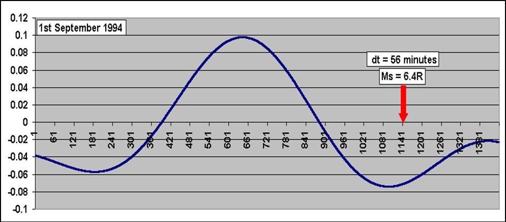
Fig. 4.1.9.4. Correlation of the EQ on 1st September 1994 time of
occurrence, with the corresponding Earth-tide.peak.
The same methodology was applied on EQs (Ms>=4.0R), which occurred
between the 1st and 22nd February 2001. Although the statistical
sample is small, it is indicative for the validity of the
methodology.
Magnitude window Ms> = 4.0 R (February 2001)
Total No. of EQs : 7
Time window : 1 hr
No. of EQs within time window : 2
P value : 0.286 or 28.6%
Time window : 2 hours
No. of EQs within time window : 5
P value : 0.714 or 71.4%
The following figures demonstrate the methodology, which is applied
on EQs of February, 2001 with a magnitude Ms >= 4.0R, except the
first one, which corresponds to the EQ that occurred in Athens.
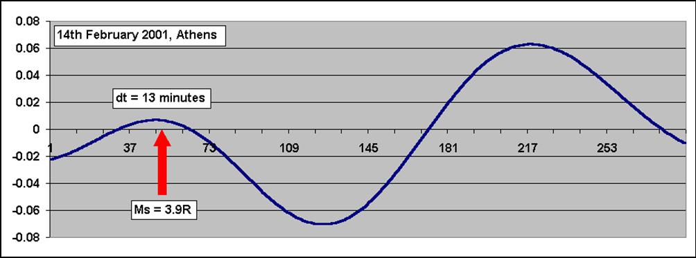
Fig. 4.1.9.5. Correlation of the EQ on 14th February 2001 time of
occurrence, with the corresponding Earth-tide peak.

Fig. 4.1.9.6. Correlation of the EQ on 14th February 2001 time of
occurrence, with the corresponding Earth-tide peak.

Fig. 4.1.9.7. Correlation of the EQ on 18th February 2001 time of
occurrence, with the corresponding Earth-tide peak.

Fig. 4.1.9.8. Correlation of the EQ on 1st Feb. 2001 time of
occurrence, with the corresponding Earth-tide peak.
When the strong correlation which is observed, between the time of
occurrence of strong EQs and the 14 days period tidal wave, is
combined with the daily, tidal variation, it facilitates the
estimation of a very narrow, predictive time-window for the imminent,
strong EQ, with very large probability.
What has been demonstrated from the previous, presented, cases is
the following:
- Earthquakes, in their vast majority, occur when the stress-strain
of the seismogenic region acquires its peak stress-strain level.
- The time of occurrence of the stress-strain charge of a
seismogenic area, is strongly correlated, to the tidal peak values
of the lithospheric oscillation.
- The time of occurrence of the tidal peaks is well known in
advance, from the analysis of the tidal gravity waves, related, to
any seismogenic area.
- Within a year’s period, strong earthquakes (if any) will mostly
take place in specific times, predefined, by the analysis of the
tidal, lithospheric oscillations.
In practice, it is postulated that, with an assumed, predictive
time window of +/- 2 days, there are only 52 specific times within a
year’s period (the weekly tidal oscillation peaks) when a strong
earthquake can occur.
Assuming a more narrow predictive time window (of +/- 2 hours),
then the number of times when a strong EQ can occur within a year
increases to:
Times = weeks x 4(+/-2days/peak)x4(daily tidal peaks)
Times of occurrence = 52x4x4 = 832.
The calculated number of times of occurrence, of a strong EQ,
within a year’s period, although it looks large, it is definitely a
“small number”, compared, to the infinite times of occurrence,
suggested, from equation (4.1.1.5) and the various, proposed, models,
in figures (4.1.1.1), (4.1.1.2), (4.1.1.3).
The procedure which has already been demonstrated, by the study of
the maxima – minima of the tidal, lithospheric oscillation, can be
represented with a Boolean “AND” operation. The infinite space of
time of occurrence solutions, suggested, by the equation (4.1.1.5)
are subjected to an “AND” operation with the space of “tidal
oscillations”. This appears in the following figure (4.1.9.9).

Fig. 4.1.9.9. The infinite space of time of occurrence
solutions (outer circle), suggested, by the equation
(4.1.1.5), is subjected to an “AND” operation with the
space (inner, shaded circle) of “tidal oscillations”
times of maximum amplitude.
Although, there is an improvement in the calculation of the
predictive time window of the occurrence of a strong EQ, this is not
enough for short-term prediction. Actually, it is not practical, at
all, in predictive terms. If there is no way to identify at which
“tidal peak”, within a year’s period, an EQ will occur, then the
entire scheme is no longer a “short-term” prediction, but it becomes
rather a “medium-term” one. This type of prediction can be treated
by the already, referred, statistical methods.
Therefore, there is the necessity to constrain further more the
“predictive time window” solutions, obtained, so far. Actually, the
target is to distinguish the “candidate” tidal peaks when a strong
EQ will occur. This may be achieved by further constraining, the
already, determined, (832) time solutions, by the properties of the
“electrical signals generating mechanisms”, which already have been
presented in section (3).
4.1.10. Electrical signals timing, compared, to
lithospheric tidal oscillations.
The electric, seismic precursory signals which are presented to
date in the seismological literature are distinguished in the
following main types:
a) SES, (Seismic Electric Signals) or “high frequency”
signals.
b) Oscillating signals, mainly of 24 hours / 14 days
period following the tidal oscillation.
c) VLP signals, (Very Long Period).
Examples of such signals have already been presented in section
(3). A thorough study of the various mechanisms which generate
electrical signals, suggests that the piezoelectric is the most
probable one. This is the only mechanism that justifies in total:
the generation of SES (signals, due to higher order derivatives of
the non-linear part of the generated potential), Oscillating signals,
(due to the oscillating component of the stress-strain of the
seismogenic area, caused, by the oscillatory effect of the Earth-tides
upon the stress-strain / piezoelectric potential curve) and the VLP
signals, (due to the total form of the generated static potential
which is caused by the large scale crystal-lattice deformation).
The correlation of such signals with the tidal oscillations will be
demonstrated through specific examples, since strong EQs are not a
routine event, thus prohibiting us to apply statistical validation
by using a large number of statistical samples.
a. SES, (Seismic, Electric Signals) or “high
frequency” signals.
SES generated by the Izmit, (17/8/1999, M=7.5) EQ,
in Turkey.
The electrical signals, which were recorded in Volos (VOL), Greece
(Thanassoulas et al. 2000) before the Izmit, EQ (17th, August, 1999,
M=7.5) in Turkey, will be the first example to be demonstrated. The
detailed study of the recordings of the Earth’s electrical field by
(VOL) monitoring site, for a period of almost three months before
the Izmit EQ, revealed the existence of high frequency (SES)
electrical signals. These signals were observed almost right from
the start (21st June, 1999) of the recording period and consequently
it is justified to accept their earlier start-up time of origin.
Samples of these signals are presented bellow. During a six months
period of recording of the Earth’s electric field, only the NS
component was recorded by VOL monitoring site. The following figure
(4.1.10.1) corresponds to the recording day on 21/06/99. This
recording was performed almost two months before the strong Izmit,
(16/8/1999, M=7.5) earthquake in Turkey.

Fig. 4.1.10.1. Electrical signals, recorded on 21 / 06 / 1999
by VOL
monitoring site, at NS direction.
Next data set corresponds to the recording day on 22/07/99. That is
almost after a month later than the previous one and almost one
month before the Izmit EQ.

Fig. 4.1.10.2. Electrical signals recorded, on 22 / 07 / 1999 by
VOL monitoring site.
Similar electrical signals have been observed in this recording,
too. Almost in the entire time of recording, are observed two
distinct signals, separated, at a certain period of time, of some
hours. Next one was recorded on 03/08/99.

Fig. 4.1.10.3. Electrical signals recorded, on 03 / 08 / 1999 by
VOL monitoring site.
The next one is a two days recording from 13 to 14/08/99. That is a
very short time, before Izmit EQ (17-08-1999) occurred.

Fig. 4.1.10.4. Electrical signals recorded, on 13 – 14 / 08 / 1999
by VOL monitoring site.
The last one (fig. 4.1.10.5) had been recorded between 17-18/12/99.
By that time, the most of the stress load of the seismogenic area
had been released and, consequently, the SES signals disappeared.
This is demonstrated, clearly, by the following figure (4.1.10.5).

Fig. 4.1.10.5. Electrical field recorded, between 17-18 / 12
/ 1999, by VOL monitoring site.
The absence of electrical signals, comparing to previous figures,
is characteristic.
Another interesting observation is that, the start time of these
signals coincides with two specific daytimes.
The first one is around 9a.m, while the second one is around 21.5
p.m. This observation was studied, in detail, by separating the
“9.0a.m” signals and the “21.5 p.m” signals in two groups (signal –
A, signal - B).
The following figure (4.1.10.6) represents the existence of
electrical signals (signal – A) as a function of time (in days),
while the vertical axis represents the startup time of each signal (in
minutes) in the span of the day of its occurrence.
In the horizontal axis of time, the earthquakes in Izmit, Athens
and Duzce are marked with a red arrow.

Fig. 4.1.10.6. Daily presence of signals – A is shown,
between 20/06 – 31/12/1999.
In the following figure (4.1.10.7), the signals - B are presented
with the same annotation.

Fig. 4.1.10.7. Daily presence of signals – B is shown,
between 20/06 – 31/12/1999.
What is clear, from both figures, is the drastic decrease of the
presence of the signals after the occurrence of Izmit EQ. On the
other hand, before Duzce EQ, of a similar magnitude to Izmit EQ, no
such signals were observed. This suggests that Izmit – Duzce regions
may be considered as a unit area, stress loaded and seismically
activated. Consequently, the generated, electrical signals were
produced by the entire, seismically active area and not only by
Izmit focal region. This is corroborated from the fact that IZMIT –
DUZCE distance is of the order of 80Km which coincides quite well
with the expected fracture length of the seismogenic fault, which is
what is more or less expected for an EQ of M = 7.5.
Therefore, when most of the stresses load of the entire area had
been released (by Izmit EQ), the rest of it was not capable of
generating similar, electrical signals. Viewing this pair of strong
EQs from the point of view of electrical signals generation
mechanism, it is a very inte-resting and spectacular, seismic event.
For both signals (A, B) the mean starting time has been calculated.
For signals (A) the mean value (MVA) was calculated as 569 minutes.
MVA = 569 minutes
(4.1.10.1)
This corresponds to a mean starting time of 9hr 29 minutes. For
signals (B), the same calculation results in a (MVB) of 1257
minutes. This corresponds to a mean starting time of 20hr 57
minutes.
MVB = 1257 minutes
(4.1.10.2)
Finally, the mean time difference in time of occurrence of the
electrical signals has been calculated, as:
MVB - MVA = 11hr 28 minutes.
(4.1.10.3)
Comparing this result to the Earth-tide components, its very close
resemblance is revealed to (K2) (lunisolar) and (S2) (principal
solar) components. A discrepancy of 4.17% has been calculated for
the (K2) component, while a value of 4.4% corresponds to the (S2)
one. The satisfactory results fit what was expected from the earlier
theoretical analysis.
In simple words, the entire Izmit-Duzce seismogenic area was at
such critically point of stress-strain charged conditions, so it
generated SES twice in a day, at the peaks of the 24 hours
lithospheric oscillation.
Below are (SES) sample signals, recorded, by (HIO), (PYR) and (ATH)
monitoring sites, and compared to the 14 days period tidal,
lithospheric oscillation local peak value.
SES signals recorded at HIO monitoring
site, compared to 14 days period tidal
lithospheric oscillation.

Fig. 4.1.10.8. SES precursory, electrical signal (in blue
circles) recorded, by HIO monitoring site, between 13 and14 May 2006
(HIO060513-14).

Fig. 4.1.10.8.a. Zoom-in of the left SES signal of fig.
(4.1.10.8).

Fig. 4.1.10.8.b. Zoom-in of the right SES signal of fig.
(4.1.10.8).

Fig. 4.1.10.9. SES precursory, electrical signal (in blue
circles) recorded, by HIO monitoring site, during the 30th May 2006
(HIO060530).

Fig. 4.1.10.9.a. Zoom-in of the SES signal of fig. (4.1.10.9).

Fig. 4.1.10.10. SES precursory, electrical signal recorded, by HIO
monitoring site on 13th August 2006 (HIO060813).

Fig. 4.1.10.10.a. Zoom-in of the SES signal of fig. (4.1.10.10).

Fig. 4.1.10.11. SES precursory electrical signal (in blue
circles) recorded by HIO monitoring site, on 5th September 2006 (HIO060905).

Fig. 4.1.10.11.a. Zoom-in of the SES signal of fig. (4.1.10.11).

Fig. 4.1.10.12. SES precursory, electrical signal (in blue
circles) recorded, by HIO monitoring site on 17th September 2006 (HIO060917).

Fig. 4.1.10.12.a. Zoom-in of the SES signal of fig. (4.1.10.12).

Fig. 4.1.10.13. SES precursory, electrical signal (in blue
circles) recorded, by HIO monitoring site, on 28th December 2006 (HIO061228).

Fig. 4.1.10.13.a. Zoom-in of the SES signal of fig. (4.1.10.13).
SES signals recorded at PYR monitoring
site, compared to 14 days period, tidal
lithospheric oscillation.

Fig. 4.1.10.14. SES precursory, electrical signal recorded, by PYR
monitoring site, on 4th August 2004 (PYR040804).

Fig. 4.1.10.14.a. Zoom-in of the (4th - 5th of August) SES
signal of figure (4.1.10.14).

Fig. 4.1.10.15. SES precursory, electrical signal recorded, by PYR
monitoring site, on 30th June, 2006 (PYR060630).
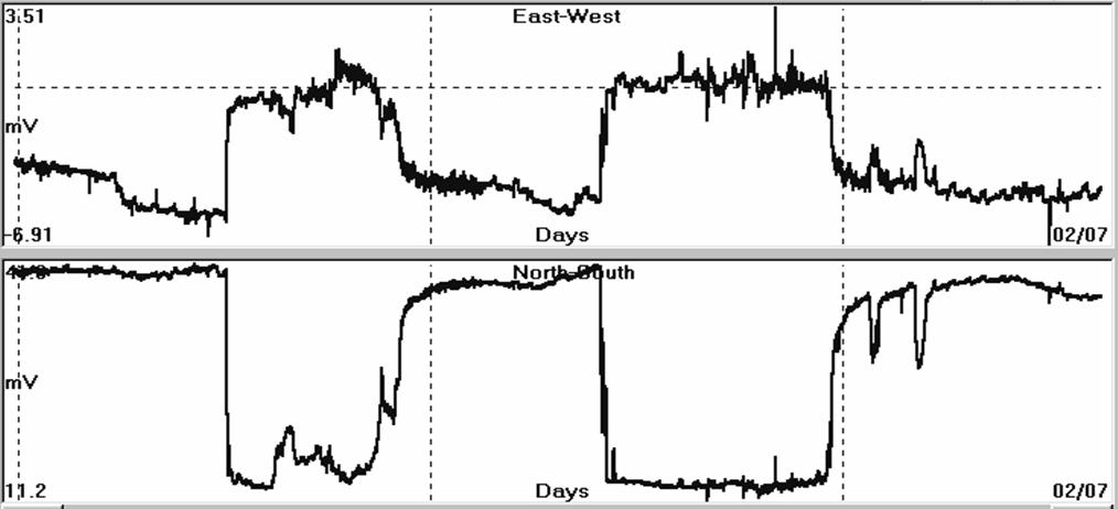
Fig. 4.1.10.15.a. Zoom-in of the SES signal of figure
(4.1.10.15).
SES signals, recorded, by ATH monitoring
site, compared, to 14 days period,
tidal lithospheric
oscillation.
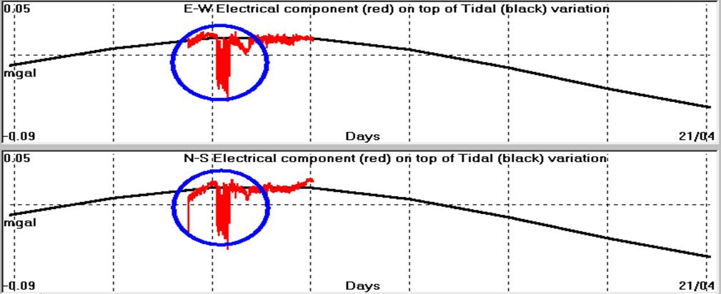
Fig. 4.1.10.16. SES precursory, electrical signal recorded, by ATH
monitoring site, on 16th April, 2003 (ATH030416).

Fig. 4.1.10.16.a. Zoom-in of the SES signal of figure
(4.1.10.16).

Fig. 4.1.10.17. SES precursory, electrical signal recorded, by ATH
monitoring site, on 20th May, 2004 (ATH040520).

Fig. 4.1.10.17.a. Zoom-in of the SES signal of figure
(4.1.10.17).
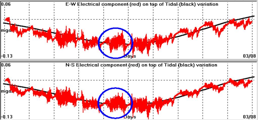
Fig. 4.1.10.18. SES precursory, electrical signal recorded, by ATH
monitoring site, on 29th July, 2004 (ATH040729).
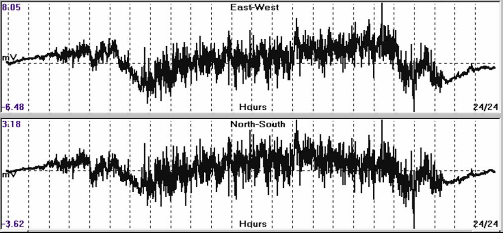
Fig. 4.1.10.18.a. Zoom-in of the SES signal of figure
(4.1.10.18).

Fig. 4.1.10.19. SES precursory, electrical signal recorded, by ATH
monitoring site, on 8th January, 2006 (ATH060108 EQ6.9).

Fig. 4.1.10.19.a. SES precursory, electrical signal recorded, by ATH
monitoring site, on 8th January, 2006 (ATH060108 EQ6.9). The red bar
indicates the time of occurrence of the 6.9R EQ (ATH060108 EQ6.9).
The previous figures (4.1.10.19 - 4.1.10.19.a) indicated the close
correlation of the EQ time of occurrence, to the 14days tidal,
lithospheric oscillation peak time and the present “coseismic” SES
signal.
It developed almost 90 minutes before the EQ occurrence and
vanished, almost 110 minutes after it. This suggests that, the
catastrophic deformation of the seismogenic area is estimated to
have lasted for about 3 hours.
In literature, and specifically in the papers which were published
by the VAN group during their research activity, a lot of SES
signals have been presented. It is worth to test the time (day) of
occurrence of these signals against the tidal lithospheric
oscillation of the 14 days period. To this end, the already
published signals which were traceable (No = 64), are tabulated in
Table - 2. The first column indicates the time of occurrence of the
SES in yyyymmdd format, while the second one indicates the time lag,
between the SES times considered as “zero” time and the time of the
tidal peak value.

The negative values, of the second column, indicate that the SES
time of occurrence follows the tidal peak”, while the positive
values indicate that the SES “preceded the corresponding, tidal
peak”.
The values, tabulated, in table (2), are presented in a graph form,
in the following figure (4.1.10.21).

Fig. 4.1.10.21. Number of SES, as a function of time lag to
tidal peak of the 14 days lithospheric oscillation are, presented.
The form of the function of SES time vs. time lag to tidal
oscillation peak times suggests that the majority of the SES occur
at some time “following” the tidal peak occurrence. By taking into
account that the stress-strain charge of the lithosphere is at
maximum load conditions during peak tidal oscillating values, then
it is justified to accept that the majority of SES are generated in
“decompression conditions” or in other words SES are “pressure
stimulated depolarization currents - PSDC” (Varotsos, 2005).
The stress-strain charge conditions where an SES may develop are
steps of sudden increase or decrease of the stress-strain load of
the lithosphere. It is worth to compare such stress-strain changes
in the lithosphere, during the preparation phases of an earthquake.
Firstly, is considered the model, proposed, by Mjachkin et al.
(1975). In this model (fig. 4.1.10.22), three characteristic phases
are present, concerning the deformation velocity during a seismic
cycle. In the first (I) phase, the seismogenic area exhibits
homogeneous cracking; during the second (II) phase, cracking
acceleration, due to interaction of cracks, is exhibited; and during
the third (III) phase, unstable cracking and main fault formation is
exhibited, and the generation of the main, seismic event follows.
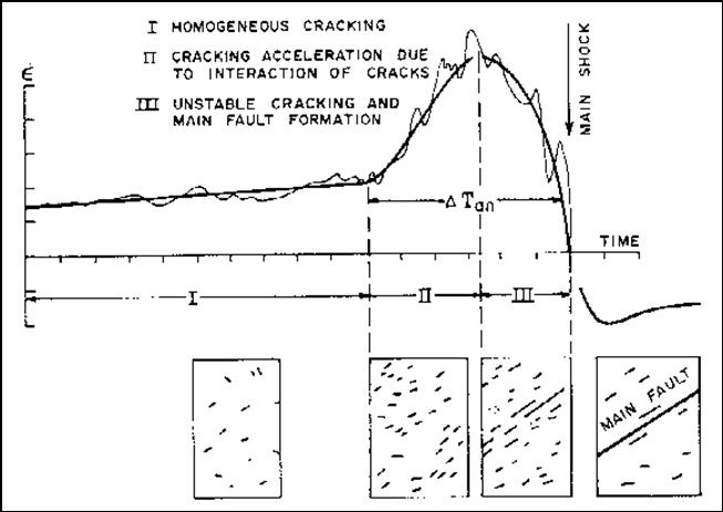
Fig. 4.1.10.22. Change of average deformation velocity, during
the seismic cycle (Mjachkin et al. 1975).
Change of stress-strain load, which can cause the generation of
SES, occurs in the boundaries between phases (I) and two (II),
between phases (II) and (III) and very shortly before the main,
seismic event. The time span of each phase is generally unknown and
therefore, even if the SES has been observed, the time window of
occurrence of the pending seismic event, is still highly
unpredictable.
The piezoelectric model will be considered next. There are two
distinct regions, where non-linear change of the strain load exists
in the strain-stress curve. In area (A), there is a rapid non-linear
increase of the strain, while in area (B), there is a non-linear
decrease of the strain. These are favorable areas, where SES can
develop either as PSPC or as PSDC.

Fig. 4.1.10.23. Areas of “comp-ressional (A) stress - strain
increase”
and ”decompressional (B) stress - strain decrease”.
These signals can be considered as of higher order derivatives of
the total piezoelectric potential generated, in terms of the
function of Piezoelectric Potential vs Time / Stress load. The
timing problem of an earthquake still exists, since the time
interval between areas (A) and (B), is still unknown.
A search, in the VAN group literature, indicates that the time of
occurrence of an SES may precede the time of occurrence of the
corresponding earthquake, from 30-240 minutes (papers of 1981) up to
11 days (papers of 1993) and probably of longer periods. The latter
is not surprising, if it is explained by the tidal lithospheric
oscillation. Actually, an SES can be generated at any favorable
tidal oscillation peak value, but the corresponding earthquake will
occur later on, when its critical stress-strain conditions are met
at a specific, future, tidal oscillation peak.
No matter what their origin is, what is important is the fact that
such signals are composed by series of short pulses in the form of
“train pulses”. A physical mechanism which can produce signals of
this kind is postulated as follows:
Let us consider the very tiny rock element, which exhibits the rock
properties of the seismogenic region. It is assumed that, this basic
element follows the stress-strain charge conditions of the entire
seismogenic area. During the boundaries of the different phases of
the Mjachkin et al. (1975) model or the areas (A) and (B) of the
piezoelectric model, this basic rock element undergoes, firstly, a
stress-strain increase, which is followed, in very short time, by a
decrease of stress-strain and fracturing, thus creating the
acceleration of cracking. Therefore, this basic rock formation
element is capable to produce, initially, a tiny PSPC, which is
followed by a PSDC before its final fracture.
Moreover, electrical signals of the same amplitude, but of
different polarity, depending on the polarity (increase or decrease)
of the stress-strain rate for the same basic rock element and for
the same rate of stress-strain charge-discharge, will be generated.
Therefore, each pair of positive-negative current pulses, generates
a “square electrical, potential pulse”, the basic element of the
“train pulse”, which exhibits a duration of a few minutes, which
depends on the time, required, to complete its “tiny seismic cycle”.
The close inspection of the SES signals, recorded by ATH, PYR and
HIO so far, indicates that a period of 8-15 minutes, but shorter
periods as well (from a few ms to a few minutes) have been recorded
by the VAN group.
Summarizing all the above, it can be said that, the SES presence is
a clear indication that an unknown seismogenic area has reached a
stress-strain level, close, to the critical stress-strain charge
conditions, which are necessary for the generation of a seismic
event. The problem that still exists, in terms of “time prediction”,
is that, there is no method (in terms of short-term prediction), to
suggest the calculation of the time to remain between the SES
occurrence and the time of the seismic event. When this seismic
event will occur, is still unknown.
b. Oscillatory type earthquake precursory signals.
The uncertainty for the timing of a future seismic event, which is
introduced: a) by the use of SES, as it was explained earlier, b) by
the use of Mjachkin et al. (1975) fracturing model and c) by the
piezoelectric model (see fig. 4.1.10.23) is resolved, in most cases,
by the study of the oscillatory component of the Earth’s electric
field. This type of component is induced by the lithospheric plate
tidal oscillation; see Section (3) and the piezoelectric model of
figure (4.1.10.23). An increase in amplitude of the Earth’s
oscillating, electric field develops and lasts all along the time
between the two regions (A) and (B). Shortly after the (B) area, the
seismic event takes place. Consequently, the presence of this type
of oscillation indicates that the seismogenic area has passed the
(A) area and approaches the (B) one, in a short time. The seismic
event occurs at the next tidal amplitude peak, of the 14 days
period, tidal, lithospheric oscillation, when the stress-strain load
is at its maximum (Thanassoulas et al. 2003). Samples of such
oscillations, along with the corresponding earthquakes that occurred
at the tidal oscillation peak, are presented in the following
figures:

Fig. 4.1.10.24. Daily tidal oscillation of the earth’s
electric field (red line on top of the 14 days period,
tidal, lithospheric
oscillation – black line, VOL monitoring site). The blue bars
indicate the time of occurrence of two earthquakes of M = 4.8R (Thanassoulas
et al. 2003)
In the first example of figure (4.1.10.24) it is evident that the
two earthquakes of M = 4.8R, which occurred in the presented period
of 16 days (1st January, 2001 – 17th January, 2001), took place
exactly on the day of the peak of the 14 days period, tidal,
lithospheric oscillation.
Moreover, both earthquakes were preceded by an increase of the
amplitude of the electric field oscillation.
In the next example (fig. 4.1.10.25) the presented time period
spans from 22nd April, 2001 to 1st May, 2001. The only one
earthquake of magnitude M = 5.3R, which took place in this period,
occurred on the peak of the 14 days period of the tidal lithospheric
oscillation.

Fig. 4.1.10.25. Daily tidal oscillation (22nd April to 1st
May, 2001) of the Earth’s electric field (red line on
top of 14 days period, tidal, lithospheric oscillation – black line, VOL monitoring
site). The blue bar indicates the time of occurrence of the M = 5.3R
earthquake (Thanassoulas et al. 2003).
In the next case (fig. 4.1.10.26), which corresponds to the period
of 11th August, 2002 to 4th September, 2002, three consecutive
earthquakes of M = 5.1R occurred, during the peak value of the 14
days period, tidal, lithospheric oscillation.

Fig. 4.1.10.26. Daily tidal oscillation (11th August to 4th
September 2002) of the Earth’s electric field (red line
on top of 14 days period, tidal, lithospheric oscillation – black line, VOL
monitoring site). The blue bars indicate the time of occurrence of
three earthquakes of M = 5.1R (Thanassoulas et al. 2003).
One more example is presented in the following figure (4.1.10.27).
In a month’s period (15th June to 13th July, 2003) one earthquake
occurred, 3 days after the peak value of the 14 days period, tidal,
lithospheric oscillation. That earthquake was preceded by an
increase of the amplitude of the Earth’s daily oscillation of its
electric field.

Fig. 4.1.10.27. Daily tidal oscillation (15th June to 13th
July, 2003 red line, PYR monitoring site) of the Earth’s electric field on
top of 14 days period, tidal, lithospheric oscillation (smoothly
oscillating black line). The blue bar indicates the time of
occurrence of the M = 5.5R earthquake.
An exceptional example is the one in figure (4.1.10.28). This
example presents Skyros earthquake case (M = 6.1R, 26th July 2001).
The main seismic event was preceded by a drastic increase of the
amplitude of the Earth’s electric, daily oscillating field, which
lasted for a few days. On 23rd July the data were presented in the
seminar organized by the INRNE, BAS, Bulgaria and following this
methodology, it was suggested (a priori), that this earthquake is
likely to happen on 25th to 26th July (after 2 days) and
specifically 20 minutes to midnight (GMT).
It was, obviously, a very strong statement, taking into account
that, in the best case, the seismological community accepts
“predictive capability” for medium term predictions only.
What followed the next two days is what was exactly expected to
happen, always according to the already, proposed, methodology. The
earthquake took place 20 minutes after midnight. The proof of this
fact is presented in the following figures. In figure (4.1.10.28) is
presented the 14days tidal, lithospheric oscillation, superimposed
by the daily, oscillating Earth’s electric field.

Fig. 4.1.10.28. Skyros EQ (26th July 2001). Fore – main - after
shocks are indicated by blue bars. 14 days tidal lithospheric
oscillation is represented by a smooth black line, while the red
line indicates the daily oscillating Earth’s electric field (Thanassoulas
et al. 2003).
The main event took place at the minimum peak of the 14 days,
tidal, lithospheric oscillation (fig. 4.1.10.29), while, during this
14 days period peak tidal value, there was, simultaneously, a daily
tidal peak value, at the time “20 minutes to midnight of 25/26th of
July”. Therefore, following the methodology, which had already been
presented, the pending earthquake, would take place, due to the
presence of the generated, strong, electrical signals:
a) at the peak of the 14 days period, tidal,
lithospheric oscillation, thus suggesting the date
25th to 26th (fig.
4.1.10.29)

Fig. 4.1.10.29. Skyros EQ (26th July 2001, M = 6.1R) time of
occurrence (red bar), correlated, to the 14 days period, tidal,
lithospheric oscillation (Thanassoulas et al. 2001b).
b) 20 minutes to midnight (fig. 4.1.10.30).
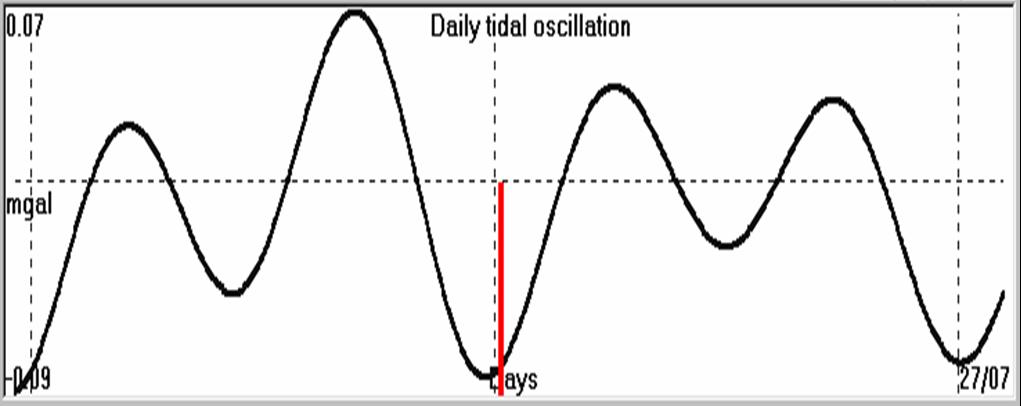
Fig. 4.1.10.30. Skyros EQ (26th July 2001, M = 6.1R) time of
occurrence (red bar), correlated, to the daily, tidal, lithospheric
oscillation (Thanassoulas et al. 2001b).
It is anticipated that for a scientist, initially, it is very
difficult to believe this prediction. In order to resolve this
unpleasant situation it was asked from the BAS organizing committee,
to validate it, in written form. The produced validation is
presented in the following page.

Some more examples of earthquakes which were preceded by an
increase of the Earth’s daily oscillating field, recorded, by PYR
monitoring site, are presented in the following figures:

Fig. 4.1.10.31. Earthquakes (M = 5R, blue bars), which
occurred one day before the 14 days period, tidal, lithospheric oscillation peak
and were preceded by a daily, oscillating earthquake precursory
signal. Recording period lasts from 2nd June to 18th June, 2003.

Fig. 4.1.10.32. Daily, tidal oscillation (24th August to 5th
September 2003) of the Earth’s electric field (rapid
oscillation) on top of the 14 days period, tidal, lithospheric oscillation
(smoothly, oscillating, black line). The blue bar indicates the time
of occurrence of the M = 4.8R earthquake.
Apart from the daily oscillating earthquake precursory signals,
other types of signals, which precede strong earthquakes, have been
observed, with much longer periods. These signals must conform to
the lithospheric, oscillatory, tidal components, triggered, by the
Sun – Moon interaction, upon the Earth. To date, the largest period
of the oscillating Earth’s electric field which has been observed,
is that of 14 days. This electrical field oscillation conforms to
the M1 (Moon declination) tidal wave. Two such cases have been
observed to date. The first one is the case of Lefkada, EQ (14th
August, 2003, M = 6.4R) in Greece and the second is the Kythira, EQ
(8th January, 2006 M = 6.9R) in Greece. These two cases are
presented in the following figures:
In figure (4.1.10.33) is presented the oscillating Earth’s
electrical field with period of 14 days.

Fig. 4.1.10.33. 14 days period oscillating Earth’s electric
field observed prior to Lefkada, (14th August, 2003, M = 6.4R) earthquake
in Greece. A red bar indicates the time of occurrence of this
seismic event.
Next figure (4.1.10.34), represents the timing of the same seismic
event in relation to the 14 days period, tidal, lithospheric
oscillation. The EQ occurred 1 day before the next tidal peak.

Fig. 4.1.10.34. Lefkada EQ (14th August 2003, M = 6.4R) time of
occurrence (red bar), in relation to the 14 days period, tidal,
lithospheric oscillation.
The very same seismic event occurred in the daily tidal minimum of
the day of its occurrence, thus, validating its strong correlation
to the tidal triggering mechanism of earthquakes.
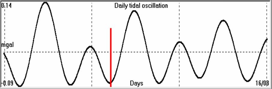
Fig. 4.1.10.35. Correlation of time of occurrence (red bar) of Lefkada, Greece EQ (14th August, 2003, M = 6.4R) to the daily,
tidal, lithospheric oscillation.
Next example refers to Kythira earthquake (8th January, 2006, M =
6.9R). In figure (4.1.10.36) is presented the oscillating Earth’s
electrical field with period of 14 days.
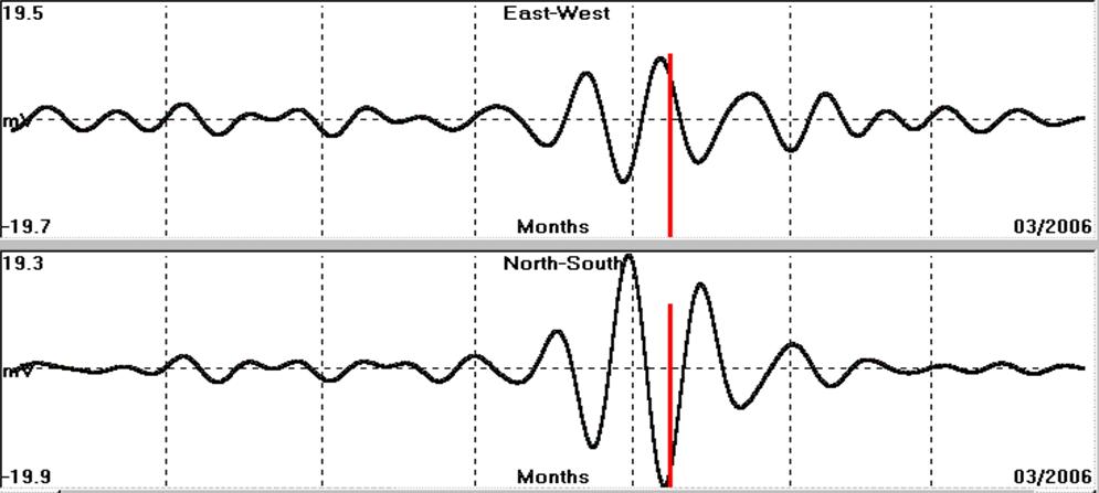
Fig. 4.1.10.36. 14 days period oscillating Earth’s electric
field, observed, prior to Kythira, (8th January, 2006, M = 6.9R) earthquake
in Greece. A red bar indicates the time of occurrence of this
seismic event.
Next figure (4.1.10.37), represents the timing of this seismic
event, in relation to the 14 days period, tidal, lithospheric
oscillation. The seismic event correlates quite well to the peak of
the 14 days, tidal, lithospheric oscillation.

Fig. 4.1.10.37. Time of occurrence of Kythira EQ (red bar) is
presented, in relation to the 14 days, tidal, lithospheric
oscillation.
The comparison of the time of occurrence of Kythira EQ with the
daily, tidal, lithospheric oscillation (fig. 4.1.10.38) indicates
its very good fit to daily, tidal minimum.

Fig. 4.1.10.38. Correlation of time of occurrence (red bar) of Kythira, EQ (8th January, 2006, M = 6.9R) in Greece, to the daily,
tidal, lithospheric oscillation.
c. VLP signals
Very Long Period (VLP) earthquake precursory signals have been
observed before strong earthquakes. Although, these signals cannot
be correlated to the 14 days period, tidal, lithospheric
oscillation, due to their very large “period”, they are warning
indicators that “some regional, large, tectonic change” is going to
take place. Whether this event ends up to a seismic event, depends
on “shorter wave length” parameters. A representative sample of such
a signal is presented in the following figure (4.1.10.40). It refers
to Kythira EQ (8th January 2006, M = 6.9R), as it was recorded by
Pyrgos (PYR) monitoring site. The recording covers (31) week’s
period of time.
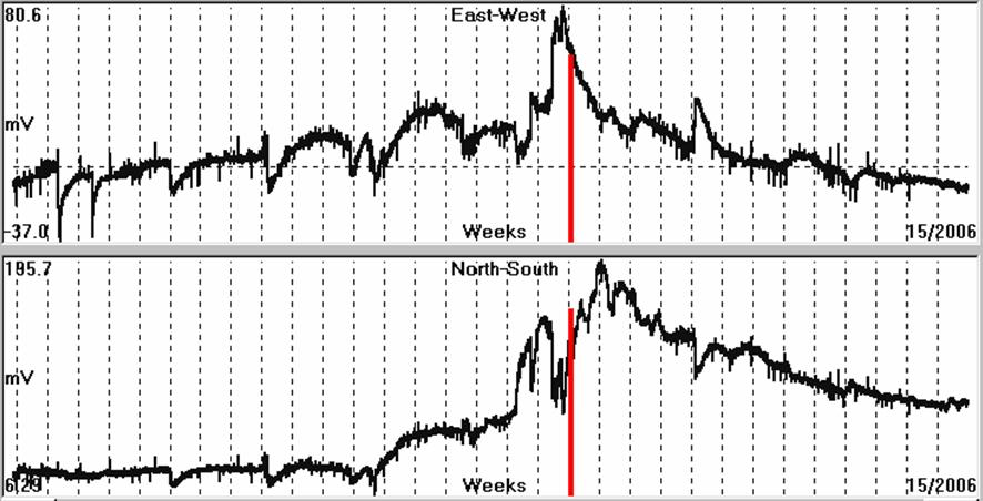
Fig. 4.1.10.40. Earth’s electric field recorded, for 31 weeks
by PYR
monitoring site. The time of the seismic (8th January 2006, M =
6.9R) event, is indicated by a red bar.
The rapid increase of its amplitude, before the seismic event, is
more evident in the NS component. After the seismic event, the
Earth’s electric field follows a slow decay, returning to its
original level. As long as the EQ occurrence time gets closer,
shorter period signals develop, which are reflected in both,
recorded, components. A three weeks recording, before the seismic
event, is shown in the following figure (4.1.10.41).
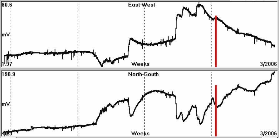
Fig. 4.1.10.41. A three weeks recording of the Earth’s
electric field by PYR monitoring site, before the seismic event in Kythira
(red bar).
The opposite polarity, observed between the two components (NS – EW),
is explained from the azimuthal direction, observed, between PYR
location and the epicentral area of Kythira EQ. The latter will be
presented, in detail, in the section, which is referred to the
“epicentral determination” of a strong EQ.
The fact that similar signals are observed even for a period of
some days is not surprising. An example of such signals is presented
in the following figure (4.1.10.42). A six days period of the
recording of the Earth’s electric field, prior to Kythira EQ, is
presented in the following figure.

Fig. 4.1.10.42. Six (6) days recording of the Earth’s electric
field, recorded by PYR monitoring before Kythira EQ time of
occurrence (red bar).
Although VLP signals, longer than 14 days period, have not been
correlated to corres-ponding longer period tidal oscillations, their
shorter wavelength content, is correlated very well. Actually, in
terms of spectral analysis, these signals provide the appropriate
oscillating components which are observed before any strong seismic
event.
Generally, the oscillating and the VLP electrical signals suggest a
generating mechanism which resembles, very close, the piezoelectric
one or “it behaves very closely to it”.
So far, the tidal triggering mechanism of the earthquakes has been
investigated and moreover it has been correlated to the generation
of seismic, precursory, electrical signals. This has an immediate
effect in the methodology, for the calculation of the timing of a
strong EQ. This is demonstrated in the following figure (4.1.10.43).

Fig. 4.1.10.43. Schematic presentation of the timing constrain of
the occurrence of a strong EQ, through the use of the tidally,
triggered, oscillating, lithospheric plate and the corresponding,
triggered mechanisms for the generation of the preseismic,
electrical signals.
The infinite number of timing solutions which result from the
mass-friction model, which is generally adopted, is further strongly
constrained through the use of the tidally, oscillating,
lithospheric plate and the very basic theory of rock mechanics,
concerning rock fracture while, finally, the short-term timing which
is required for the EQ prediction, is achieved through the
incorporation of the seismic, precursory electrical signals, at its
final stage.
At this stage, the steps to be followed, as far as it concerns the
utilization of the “short-term” time prediction of a strong EQ, are
as follows:
a. Continuous VLP monitoring and evaluation of any
“anomalous” signal, observed.
b. Continuous monitoring of SES signals. These signals
indicate that “critical” strain-
stress charge” conditions of the lithosphere have been reached.
c. Continuous monitoring of 14 days period, electrical
field oscillation, as far as it concerns
their presence and amplitude increase.
d. Continuous monitoring of 1 - day period, electrical
field oscillation, as far as it concerns
their presence and amplitude increase in relation to the 14days
period, tidal oscillation.
The most probable time of occurrence of the pending, strong EQ will
be the one that meets the criteria, already presented, in this
analysis.
The increase of the daily oscillation of the Earth’s electric
field, prior to the next to come 14-days period, tidal oscillation
peak value, has been proved the most effective one, in terms of
short-term earthquake prediction. The cases of Skyros (M=6.1) and
Kythira (M=6.9) EQs are characteristic examples, for which a
prediction time, with an error less than an hour (!), was estimated,
always following the presented methodology.
In a real time application of the methodology, it is evident that
the more the observations for analysis are available, from a widely
expanded monitoring network, the better results will be achieved.
In conclusion, the time of occurrence of a strong EQ can be
predicted, within a very narrow “time window” thus, justifying the
use of terms of: either “short term” or “immediate” prediction.
|
