Short-term Earthquake Prediction Based on Seismic Precursory Electric  Signals Recorded on Ground Surface.

3. GENERATION OF SEISMIC PRECURSORY ELECTRIC SIGNALS

Introduction

     Two methodologies are mainly followed in the scientific research. The first one observes the data which are related to a natural phenomenon and then, by analyzing them, a theoretical model that justifies the physical observations, is postulated. On the other hand, a theoretical model derives, as a result of a mathematical analysis and a search initiates in nature, so that, are found observations and data, to validate the theoretical model.
   In the case of earthquake prediction and, specifically, when we refer to the electrical earthquake precursory signals, the first case – from observations to theory – has been followed.
   Although in the recent 2-3 decades of years, has increased, actually, the number of the research papers which deal with the connection of Earth currents to earthquakes, this knowledge is not a new one. A deep research in the scientific literature has revealed that similar observations have been made, in a simpler form than nowadays, since 1692. The earliest paper that was traced is that of Milne (1890), where a large number of such events were reported.
   In chronological order, some more similar research papers are referred to, as follows:
  Terada (1931) presented a paper studying luminous phenomena, which were generated by strong electrical fields, accompanying earthquakes.
  Fedotov et al. (1970) reported anomalous, electric signals, standing well above the background of ionospheric variations, with period from a few minutes to tens of minutes and amplitudes of 50mV/Km, which preceded the M=7.9R, 1968 Japanese earthquake.
   Sobolev (1975), Sobolev et al. (1972) reported anomalous changes of the electric field of the order of several days, in an attempt to forecast, in short term, the Kamtchatka area earth-quakes.
   Varotsos et al. (1981) presented observations of the so-called seismic electrical signals, produced, by the piezostimulated currents.
   Thanassoulas (1982) reported the observed, anomalous, oscillating period of 24h, component with exponentially increasing amplitude of the electrical field of the Earth, which preceded a few days before the M=6.9R earthquake (10/01/1982) in Greece.
   Nayak et al. (1982) presented SP anomalies, observed some days prior to the occurrence of strong EQs in India.
   Varotsos et al. (1982) observed transient changes of the telluric field of the order of 0.5 – 30 mV/50m, relating to aftershocks of the strong main shock that occurred in Greece, in 1981.
   Ralchovsky and Komarov (1988) related the periodicity of the Earth’s electric field prior to strong earthquakes.
   Meyer and Pirjola (1986) observed periodic anomalies, period of 24h, in the electrotelluric field prior to a strong, imminent, earthquake in Greece.
   Miyakoshi (1986) reported anomalous time variation, of the self-potential, in the fractured zone of an active fault, preceding the earthquake occurrence.
   Thanassoulas and Tselentis (1986) reported results, concerning the oscillations (24h period) of the Earth’s electrotelluric field, observed, before strong EQs, which occurred in Greece, in 1982 and 1986.
   Meyer and Ponomarev (1987) observed a striking, electrotelluric anomaly, 6 days before an M=5.7R earthquake in the Kamchatka area.
   Thanassoulas and Tselentis (1993) reported results concerning the oscillations (24h period) of the Earth’s electrotelluric field, observed, before the strong EQs, which occurred in Greece, in1982 and 1986.
   Ifantis et al. (1993) observed long-term variations of the Earth’s electric field, preceding two earthquakes in Greece.
  Tselentis and Ifantis (1996) observed gradual variations of electric field, related to earthquakes, registered, during a 3-year independent investigation in Greece.
   Enomoto et al., (1997) registered in Japan, pulse-like, geoelectric signals, possibly related to recent, seismic activity.
   Thanassoulas and Tsatsaragos (2000) reported, observed, oscillations of 24h period prior to Izmit (17-08-1999, Ms=7.5R) and Athens (07-07-1999, Ms=5.9R) earthquakes.
   Fujinawa et al. (2000) studied electromagnetic field anomalies (transient self-potential TSP), associated with the seismic swarm in Central Japan in 1998.
   Zlotnicki et al. (2001) observed change in frequency spectral properties of an ULF electromagnetic signal, around the 21st July 1995, M=5.7, Yong Deng (China) earthquake.
   Eftaxias et al. (2001), studied the signature of pending earthquake (Athens 1999), from electromagnetic anomalies.
   Gladychev et al. (2001) presented a study of electromagnetic emissions, associated with seismic activity in the Kamchatka region.
   Karakelian et al. (2002) analyzed the Ultra-low, electromagnetic field measurements, associated with the M=7.1, Hector Mine, California, earthquake sequence in 1999.
   Nagao et al. (2002) studied the electromagnetic anomalies, associated with Kobe earth-quake in 1995.
   Karakelian et al. (2002) observed relation of the ultra-low, electromagnetic signals, registered to the Mw=5.1 San Juan Bautista, California earthquake in 1998.
   Honkura et al. (2002) reported small electric and magnetic signals, observed before the arrival of the seismic wave, generated by Izmit, Turkey, M=7.5, earthquake.
   Pham et al. (2002), studied the anomalous transient electric signals (ATES) in the ULF band, in Lamia region (Central Greece) and an explanation was presented, referring to their generation.
   Thanassoulas and Klentos (2003) calculated the predictive parameters (time, location, magnitude) of Saros EQ M=5.4R, 2003, through the recordings of the Earth’s electrical field in Athens and Pyrgos monitoring sites.
   Hattori et al. (2004) studied the ULF geomagnetic anomaly, associated with the Izu Islands earthquake swarm, Japan in 2000.
   Ida and Hayakawa (2006), applied fractal analysis on ULF data recorded during the Guam earthquake, 1993, to study prefracture criticality.
   Varotsos (2006) presented recent, seismic, electric signals (SES) that preceded two recent strong earthquakes, in Greece.
   The literature, mentioned, earlier, is a small part of the plethora of papers, which exist in the worldwide, seismological, scientific journals and refer to the generation of earthquake precursory, electrical signals.
   On the other hand, a limited number of papers which strongly object the validity of the generation of such electrical, seismic, precursors exist, too. In contrast to the 30 papers, listed above, which are in favor of the generation of seismic, electric precursors, only a very small number was traced against, as follows:
   Gruszow et al. (1996) suggested that the SES, recorded, by the VAN group and corresponding to Kozani, Greece earthquake (M=6.6, 1995) was of artificial origin.
   Variemezis et al. (1997) concluded that Earth’s electric field recordings could not be evaluated as earthquake precursors, because of the high seismicity level of the area of the study (Thessaly, Central Greece).
   Bernard et al. (1997) suggested, that the SES signal, recorded, by the VAN group in Volos monitoring site and, related, to the Aigion earthquake (M=6.2, 1995), was probably generated by a source, located, near the monitoring site, 100Km away, whatever its correlation with the earthquake. In other words it was a local event.
   Pinettes et al. (1998) suggested that the source of the SES on 30th April, 1995, recorded, by the VAN group, is very unlikely to be located in the hypocentral zone of the Aigion, Greece earthquake in 1995, whatever its actual link with the earthquake.
   Pham et al. (1999) after analyzing SES signals, recorded, at Ioannina area, Greece, concluded that some of the signals, recorded, at this site and, identified, as SES, are probably of artificial origin, and that the criteria, used, by the VAN group, are not sufficient to guarantee that, the so-called SES, are not man-made.
   Variemezis et al. (2000) studied the telluric field of the Earth in Thessaly (Central Greece). A correlation of the characteristics of the telluric field with the earthquake magnitude was attempted, but no reliable relationship was obtained.
   Pham et al. (2001) attributed the origin of SES to the leakage of electric and phone networks of the CRG (Research Centre for Geophysics, Garchy (Nievre), France.
   Pham et al. (2002) suggested that the SES, recorded, by the VAN group at Lamia area, Greece, were of anthropogenic origin.
   A different group of papers deals with physical mechanisms, which can cause the generation of electrical currents and therefore, electrical fields in the Earth. These are mainly triggered by the dilatancy of the focal region.
   Some of the main, physical mechanisms which may generate electrical precursory currents - signals follow:
 

3.1. Streaming - electrokinetic potential model (Mizutani et al. 1976, Corwin,R.F., and Morrison, H.F. 1977, Fitterman 1978, Dobrovolsky et al. 1989, Gershenzon et al. 1989 Ger-shenzon et al. 1990).
   In this model, the streaming-electrokinetic phenomena are postulated, as a physical mechanism which generates electrical potential, caused, by diffusion of fluid into a dilatant, focal region. The details of this mechanism are demonstrated in the following figure (3.1.1).

Fig. 3.1.1. Schematic diagram of electric double layer and velocity profile utilized, in a capillary (after Mizutani et al. 1976).

   The streaming potential E is given by the equation:


                                                   grad E = -εζ/ησ grad P                                                               (3.1.1)


   where: (σ) and (P) are the electrical conductivity and the pressure of the fluid, (ε) is the dielectric constant of the fluid, (ζ) is the zeta potential and (η) is the viscosity of the fluid.
 

3.2. Perturbation of the electric current by a resistivity anomaly (Honkura, 1976).
   In this model it is assumed that a spatially, uniform current is induced in an otherwise, uniform medium Earth. The change of the medium resistivity (due to dilatancy in the focal area), perturbs the uniform current flow and therefore, an anomalous, electrical field, is generated.
   Changes in amplitude and direction of the magnetotelluric field seem to be observable and could be used for earthquake prediction methodologies.
 

3.3. Single rock fracturing model, (Ogawa et al. 1985).
   In this model, the abrupt split of the crystal lattice of the rock formation, in the lithosphere, results, temporarily, in charge separation and movement. This corresponds, momentarily, in a current pulse generation and therefore, electrical signal generation.

   Moreover, some more mechanisms may be activated during this process such as a) contact electrification, b) triboelectricfication, c) streaming electrification, and d) piezoelectricity.
 

3.4. Piezostimulated model (Varotsos 2005, Varotsos and Alexopoulos 1984a, 1986).
   In this model, sub-critical stress level variations, applied, at the lithosphere, are capable of triggering emissions of piezostimulated currents (PSC). This mechanism is illustrated in the following figure (3.4.1).

Fig. 3.4.1. The piezo-stimulated current j (drawing c), flows during a stress accumulation stage (drawing b) at a critical stress level Pσcr,, which is smaller than the fracture stress of rocks Pσfr, while the external electric field E (drawing a) , is kept constant. The electric dipoles (drawing d) well before Pσcr, are, randomly, oriented, while approa-ching the Pσcr, become cooperatively, oriented. Drawing c indicates that “points” obeying the condition P = Pσcr, lay on a surface A (drawing e) that sweeps through the stressed volume V (Varotsos, 2005).

3.5. Piezoelectric model (Thanassoulas et al.1986).
   In this model, the presence of quartzite in the crust is the very basic element of the mechanism (Ringwood 1959, 1966). The form of the strain load, applied, on the lithosphere, triggers the generation of piezoelectric phenomena.
   The Earth-tides modulate the strain load of the lithosphere and therefore, various types of electrical signals, are generated. This mechanism is illustrated in the following figure (3.5.1).

Fig. 3.5.1. The upper graph represents the piezoelectric potential, generated, as a function of the stress load, and applied, in the focal region. The middle graph represents the first derivative of the simultaneous, total static field, generated, while the lower graph represents (in absolute values) the electrical signals, which are generated by the nonlinearity that exists at the start and at the end parts of the total stress-potential curve.

   This mechanism, consequently, justifies the generation of three types of electrical signals:

      a) an oscillatory type electrical signal, closely, related, and, triggered by, the Sun – Moon

          tidal  waves at various tidal periods,

      b) a plateau-type signal, generated, by the derivation of the total piezoelectric field, which

          is generated by the total stress load of the focal area,

     c) a higher derivative electrical signal, generated, during the non-linear stage of the focal

         area stress load – deformation at the start and end of the total host rock fracturing

         phenomenon.

   It is worth to mention that piezoelectric potentials, generated, by quartzite crystal lattice deformation, exceed by many orders, in amplitude, any other physical mechanism which can generate electrical potentials through any other possible methodology, observable, in nature.
 

3.6. Ionospheric induction model (Meyer, K., and Teisseyre, R., 1988).
   In this model, the steady state, oscillating, ionosphere induces oscillating current in the ground. The developed Earth potential (V=I*R) amplitude increases, as long the resistivity of the dilatant region increases, due to preparation processes that take place before a strong EQ. The net result is an oscillating field with continuous amplitude increase, towards the time of occurrence of the imminent EQ. This mechanism is presented, schematically, in the following figure (3.6.1).

Fig. 3.6.1. Electric field of increasing amplitude (middle graph) Induced, due to ionospheric oscillation (upper graph) and increase of resistivity (lower graph) of the focal region (Meyer and Teisseyre, 1988).

3.7. Local piezoelectricity activation (Sornette and Sornette, 1990).
   According to this model, randomly, oriented, piezoelectric crystals, present in the crust, under the application of a sufficiently large stress load, are reoriented, thus acquiring the behavior of a single, large crystal. This is a phenomenon arising from local, cooperative configurations in the host medium.
 

3.8. Displacement of charged dislocations (Slifkin 1993, Lazarus 1993).
   In this mechanism, the generation of electrical signals, is the displacement of segments of charged dislocations, responding to changes in applied stress. In other words it is “the plastic deformation of ionic solids, present, in the Earth’s crust. The resistivity of such solids is quite high, so that large electrostatic signals may be generated with essentially, no concomitant currents”.
 

3.9. Potential gradients generated, due to presence of long-range stress (Gersherzon et al. 1993).
   This mechanism suggests that, a long range stress field which occurs before a strong earthquake gives rise to electrical potential gradients over heterogeneous ground, in large distances.
 

3.10. Magmatic mechanism of shallow crustal EQ preparation (Guterman 1994, Rokityansky, 1999).
   This model consists of a mantle chamber, the central crustal magma chamber and the interconnecting each other magma channel. A more generalized model is shown in the following figure (3.10.1).

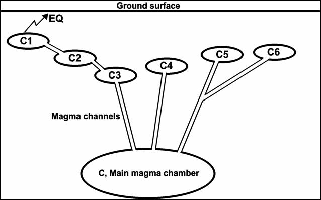
Fig. 3.10.1. A main, deep, large, magmatic chamber feeds shallower and smaller magmatic chambers, with magma, through the interconnecting channels (after Rokityansky, 1999).

   Probably, the generation of electrical signals can be connected, with the beginning of magma flow and the opening of magma channel(s).
 

3.11. The deformation induced, charged flow (DICF model), (Nowick 1996, Varotsos et al. 2001c).
   According to this model, a crystal is capable of generating a transient, electric current flow, as long as it is inhomogeneously, deformed, even in the absence of an external, electric field. This mechanism was firstly studied in laboratory conditions on NaCl crystals by Nowick (1996).
 

3.12. Pulsed charge model (Ikeya et al., 1997a, b).
   Following this model, quartz-bearing rocks, in the fault area, generate electric pulses, due to the presence of electric dipoles. The SES signals, observed, by the VAN group, are considered as the envelope of these electromagnetic pulse waves.
 

3.13. Multiple fractures model (Morgounov, 2001).
   Multiple micro fractures, which occur during the final phase (tertiary creep under stress relaxation) of the preparation of a strong EQ and in the time of focal deformation, produce electrical pulses, shown in the following figure (3.13.1).

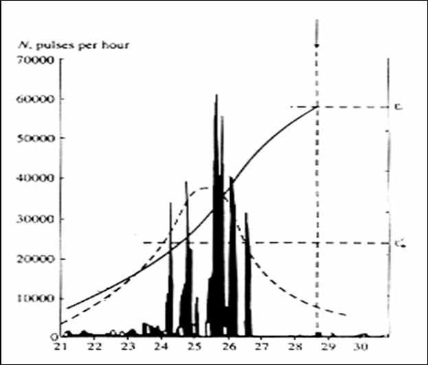
Fig. 3.13.1. Increase of the generation of electrical pulses, during the stage of tertiary creep and acquiring by the focal area the property of irreversibility (after Morgounov, 2001).

3.14. Electromagnetic emission model, related to dislocation dynamics (Teisseyre, 2001d).
   According to this model, dipole polarization and the motion of charged dislocations are combined under the influence of the evolving field stresses, along with the charge emission which takes place in the processes of micro fracturing, as well as the emission of exoelectrons and the positive hole carriers.
 

3.15. Triggering of positive hole-pairs - PHP, (Friedemann, 2002).
   Generally, when minerals crystallize in an environment rich of H2O, then positive hole-pairs (PHP) are introduced in their crystalline lattice. When these PHP acquire mobility, which is due to micro fracturing, they form rapidly moving, charge clouds which may account for the earthquake, related, electrical signals and EM emissions.
   Probably in the future, some more physical mechanisms, capable of generating seismic, precursory, electrical signals, will be found or have already been found, but it was not easy to detect them in the worldwide literature, available, on this topic. For those, who are interested in mathematical and physical details on the mechanisms already presented, the monograph “The Physics of Seismic Electric Signals”, written by Varotsos (2005), is highly recommended.
   Some general comments must be made, concerning the mechanisms which are capable of generating electrical signals and their properties, too.
It must be pointed out that, not all these mechanisms are triggered during the process of the preparation of a strong earthquake. In practice, it is not known at all if any specific mechanism has been triggered or some of them have been initiated, either simultaneously or in different time periods. Moreover, different strong earthquakes, generally, trigger different physical mechanism(s), which depend on the tectonic and geological regime of each seismogenic area.
   A common feature of all, the presented mechanisms, is their dependence on stress increase in the seismogenic area. Additionally, since the stress of the Earth’s crust is affected by the tidal variations, the tidal stress load will initiate these mechanisms, too.
A valid physical mechanism, capable of generating electrical signals must justify, at least, some of the different kinds of earthquake precursory, electrical signals, which have been observed and reported by different researchers of this topic, or all of them in a favorable case.
   Although the, presented, generating mechanisms are based in different physical bases, in a macroscopic mode of observation, they exhibit a piezoelectric behavior (Varotsos, 2005).
The earthquake precursory, electric signals are, as a rule, activated, at a certain time, before the occurrence of a strong EQ. The actual time, before the earthquake occurrence, depends on the electric signal type, the physical mechanism(s), triggered, and the magnitude of the pending earthquake. It is well understood that it takes longer for a strong earthquake to prepare, than it takes for a smaller one.
   As far as it concerns the propagation distance of the seismic, electric, precursory signals, it must be pointed out that the Earth behaves as a low pass filter and therefore, high frequency electrical signals, generated, in the focal area, are drastically attenuated in short distances from it. On the contrary, low frequency, electrical signals (with periods larger than say 1-2 minutes) are capable of distant propagation (Varotsos, 2005). This is explained by the crust resistivity model, presented in figure (2.4.4). Such a case was observed, as far as it concerns the Izmit, Turkey earthquake in 1999 (17th August, M=7.5R), when electrical, precursory signals were recorded in Volos area, Greece (Thanassoulas et al., 2000), at a line distance of almost 650Km from Izmit epicentral area.
 

3.16. Seismic, precursory, electrical signals samples.

   A logical step, next to what has been already presented and concerning the generation mechanisms of the preseismic, electrical signals and the signals themselves, is to present representative samples of continuous recordings of the Earth’s electric field, over rather long time periods. In this way, the entire issue of the “normal” Earth’s electric field, as well as the anomalous “seismic, precursory, electrical signals”, will become clearer to the reader.
   Presentation of typical examples of the Earth’s electric field, recorded, by Athens (ATH), Pyrgos (PYR), Volos (VOL) and Xios (HIO) monitoring sites in operation in Greece, follow. When necessary, explanations for each drawing are given.

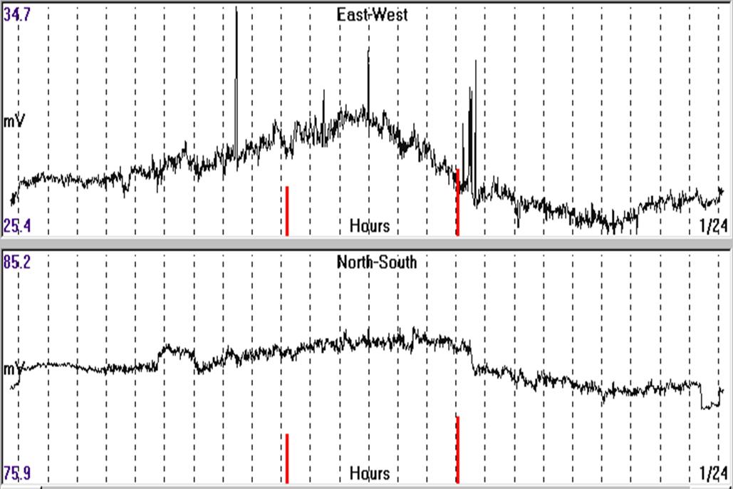
Fig. 3.16.1. Daily variation of the Earth’s electric field (29th December, 2006), recorded by ATH monitoring site.

   A daily tidal variation (fig.3.16.1) is distinguished on the EW component of the electrical field. Apart from the distinct spikes, recorded, this is considered as a rather typically “quiet” day in terms of “anomalous, precursory, electrical signals”. Typical “white” noise amplitude is of the order of a fraction of a millivolt. The red bars indicate the time of occurrence of earthquakes with a lower threshold magnitude of M = 4R (scale max. M = 8R).
Next let us consider a longer period of seven (7) days. This is presented in the following figure (3.16.2).

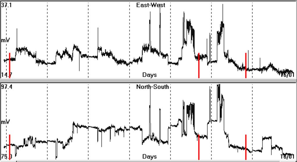
Fig. 3.16.2. Variation of the Earth’s electric field for a period of seven days (10th-16th January, 2007), recorded by ATH monitoring site.

   In this case, the lower threshold magnitude of the indicated earthquakes is: M = 4.5R. It is obvious that the “noisy” character of the recording increases from left to right of the drawing, while after the occurrence of the two right most seismic events, it becomes again close to normal. Moreover, sudden large electrical field offsets exist in the recording, superimposed by some shorter period rapid, electrical pulsations (14-15th January, 2007)
An even longer period (thirty (30) days) is presented in the following figure (3.16.3). The main philosophy, behind this presentation, is to familiarize the reader with the issue of the terms “normal recording” and “noisy recording”.

Fig. 3.16.3. Variation of the Earth’s electric field recorded, for a period of five weeks (16th December 2006 –17th January 2007), by ATH monitoring site.

   In this case, the lower threshold magnitude of the indicated earthquakes is: M = 5.0 R. The tidal character of the oscillation of the Earth’s electric field is clearly presented, mostly in the EW component of it.
   Moreover, become visible variations of the Earth’s electric field, with duration of the order of some days.
   A six months period recording of the Earth’s electric field, is presented in the following figure (3.16.4).

Fig. 3.16.4. Variation of the Earth’s electric field recorded, for a period of six (6) months (18th July 2006 – 17th January 2007), by ATH monitoring site.

   In this case, the lower threshold magnitude of the indicated earthquakes is: M = 5.6 R. The large anomaly, observed, at the start of November 2006, was followed by an earthquake of M = 4.0R that occurred a few Km away from the location of ATH monitoring site. An interesting characteristic of the recording, in this presentation, is the gradual decrease of the Earth’s electric field amplitude.
   In figure (3.16.5), a twelve (12) months period recording is presented. The entire data spans from 25th December 2005 to 17th January 2007.

Fig. 3.16.5. Variation of the Earth’s electric field recorded, for a period of twelve (12) months (25th December, 2005 - 17th January, 2007), by ATH monitoring site.

   A lower threshold magnitude, as M = 6.0 R, has been adopted in this case, for the indicated earthquakes.
   Actually, the one indicated, is the East Kythira, earthquake (M=6.9R) in Greece. The first half of the period of the Earth’s electric field recording is mostly stable, while at the second half a gradual increase is observed. At the end of this recording period, a tendency of amplitude decrease is more visible in the EW component.
Finally, the entire recording of the Earth’s electric field is presented (fig.3.16.6) for the total time of operation of ATH monitoring site (15th April 2003 – 17th January 2007), that is nearly four years of operation.

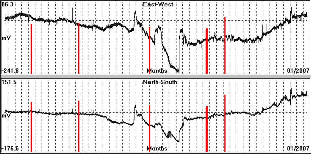
Fig. 3.16.6. Variation of the Earth’s electric field recorded, for a period of about four (4) years (15th April, 2003 – 17th January, 2007), by ATH monitoring site.

   The same, as previously, lower threshold magnitude of M = 6.0 R, for this case, has been adopted for the indicated earthquakes. In a similar way the recordings from the monitoring sites of PYR (fig. 3.16.7) and HIO (fig. 3.16.8) are presented as follows:

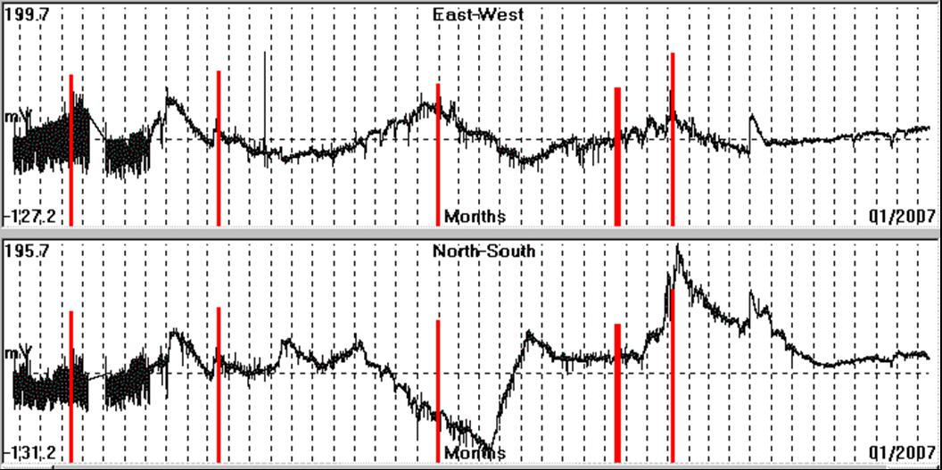
Fig. 3.16.7. Variation of the Earth’s electric field recorded, for a period of about four (4) years (23rd May, 2003 – 17th January, 2007), by PYR monitoring site.

   A characteristic feature in the previous recording is the yearly oscillatory character of the Earth’s electric field, observed, mainly in the EW component of it.

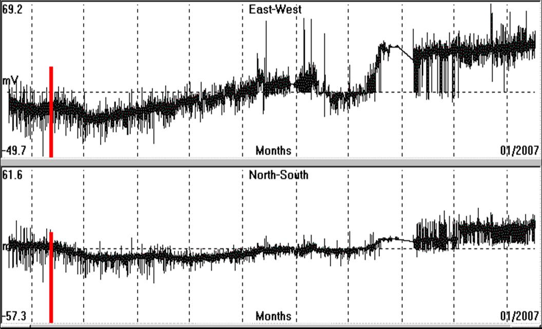
Fig. 3.16.8. Variation of the Earth’s electric field recorded, for a period of about eleven (11) months (18th March, 2006 – 17th January, 2007), by HIO monitoring site.

   From all these recordings, it is obvious, that the amplitude of the variations of the Earth’s electric field increases, as long as its period increases. Starting from a variation of the order of a few millivolts and for a duration of less than an hour (fig. 3.16.1), the observed, electrical variations range up to 330 mV p-p, as in the case of PYR monitoring site (fig. 3.16.7), for a period of about ten (10) months.
   The generalized form of the Earth’s electric field which has been recorded in three different monitoring sites for a certain period has been presented, so far. No special reference has been made for as it concerns the occurrence of strong earthquakes and the actual earthquake electrical precursory signals which preceded them. Such electric signals, which preceded actual strong earthquakes, will be presented, in the figures to follow.
   These signals are categorized as follows:


   Seismic, electric signals (SES), initially, observed by the VAN (Varotsos et al. 1981) group,


   Daily oscillations of the Earth’s electric field, initially, observed by Thanassoulas (1982),


   Very long period – of some days or months – variations, initially observed by Sobolev

   (1972, 1975).
 

3.16.1. SES precursory, seismic, electric signals samples have been presented, in many publications of Varotsos et al. These signals consist of train-pulses of some minute’s duration.
Their overall duration is of the order of 1 – 2 hours. The amplitude of these signals stands well above, the background noise of the monitoring site. Some typical examples are presented in the following figures:

Fig. 3.16.1.1. SES recorded by IOA (1988) and VOL (1995) monitoring sites of VAN network (Varotsos et al. 1996).

Fig. 3.16.1.2. SES recorded by VOL (2001) monitoring site of VAN network (Varotsos, 2005).

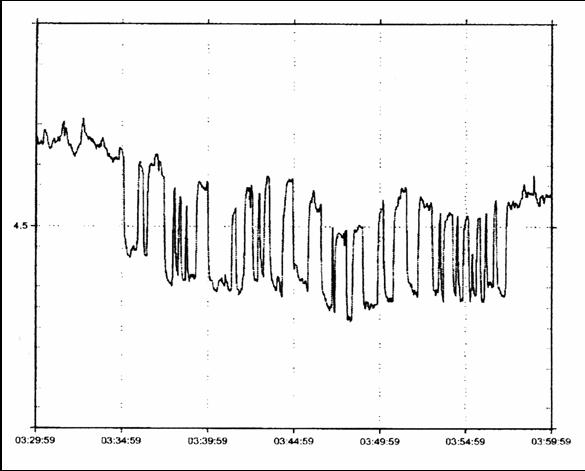
Fig. 3.16.1.3.  SES recorded by ROD (2003) monitoring site of VAN network (Teisseyre et al. 2004).

Fig. 3.16.1.4. SES recorded by PIR (2004) monitoring site of VAN network (Varotsos et al. 2006a).

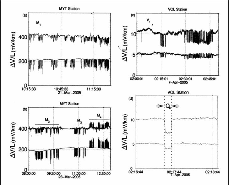
Fig. 3.16.1.5. SES recorded by MYT (2005) and VOL (2005) monitoring sites of VAN network (Varotsos et al. 2006b).

   Thanassoulas et al. (2003), recorded similar precursory, seismic, electrical signals. The following figures present such signals, thus, is fulfilled the very basic principle, required by the scientific research that is “the experimental data of any experiment must be reproducible from any other independent researcher”.

Fig. 3.16.1.6. SES recorded by VOL (2002) monitoring site.

   It must be pointed out that in Volos area, Greece, the VAN group operates a monitoring site (VOL) of the Earth’s electric field, while at the same time a different monitoring site, close to Volos area, but at a distance of a few Km is operated by an independent private researcher.

Fig. 3.16.1.7.  SES recorded by ATH (2003) monitoring site.

   Similar signals were recorded by HIO monitoring site, which was installed on Hios Island, East Greece, early of the year 2006.

Fig. 3.16.1.8. SES recorded by HIO (2006) monitoring site.

Fig. 3.16.1.9. SES recorded by HIO (2006) monitoring site.

Fig. 3.16.1.10. SES recorded by HIO (2006) monitoring site.

Fig. 3.16.1.11. SES recorded by HIO (2006) monitoring site.

Fig. 3.16.1.12. SES recorded by PYR (2004) monitoring site.

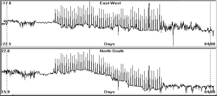
Fig. 3.16.1.13. SSES recorded by PYR (2004) monitoring site.

   A very interesting SES signal, is the one that preceded East Kythira, earthquake (M = 6.9 R) in Greece (2006). Actually, this signal was recorded by ATH, preceded the occurrence of the earthquake, for almost 1.5 hours and lasted for almost the same time after it. This is presented in the following figure (3.16.1.14).

Fig. 3.16.1.14. SES recorded by ATH, almost concurrently with East Kythira, earthquake (red bar, M = 6.9 R) in Greece (2006).

   Slightly different types of seismic, precursory, electrical signals are these, presented by Morgounov (2001). These signals consist of large electrical spike-like noise which precedes the main, seismic event for a long period (sometimes even months). The first presented, example, refers to Izmit, earthquake (M = 7.5R) in Turkey (1999), demonstrated in the following figure (3.16.1.15).

Fig. 3.16.1.15. Spike-like electrical signals, recorded for a period of a few days prior to Izmit, earthquake (red bar, M = 7.5 R) in Turkey (1999) at a distance of about 650Km by VOL monitoring site.

   Similar, spike-like electrical, precursory signals were recorded by PYR (2003) monitoring site. The red bar indicates the time of occurrence of the seismic event. This is presented in the following figure (3.16.1.16).

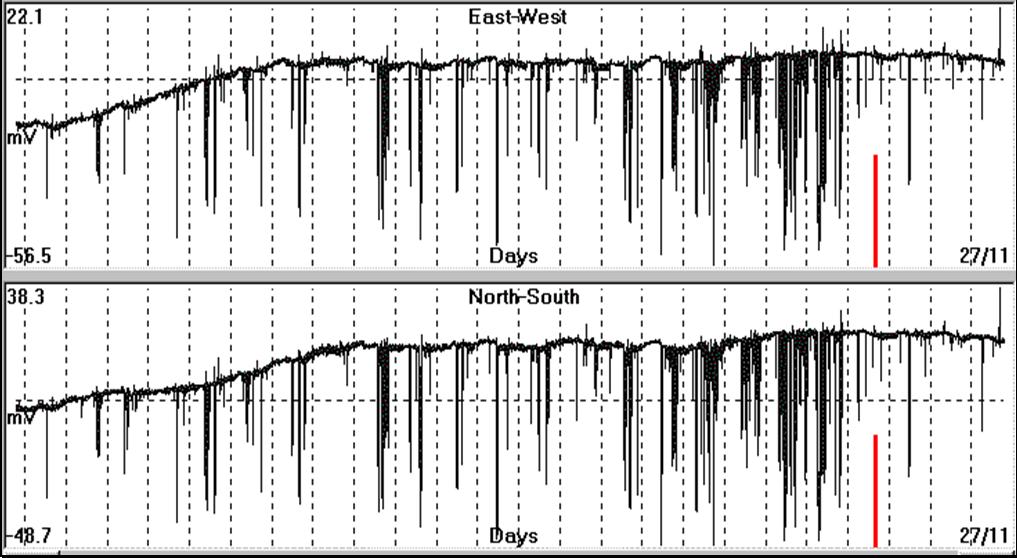
Fig. 3.16.1.16. Spike-like seismic, precursory, electrical signals, recorded by PYR (2003) monitoring site, prior to the main seismic event (red bar).

3.16.2. Oscillatory type earthquake precursory, electric signals, with a period of 24 hours, were initially, reported by Thanassoulas (1982). In the scientific literature, referring to the topic of earthquake prediction, just a few papers appeared on the same topic in the decade of 80’s – 90’s, which presented, too, a generating mechanism, justifying the presence of these signals (Thanassoulas et al. 1986;1993, Meyer et al. 1986; 1987; 1988, Ralchovsky 1988). Examples of such signals are presented in the figures to follow.

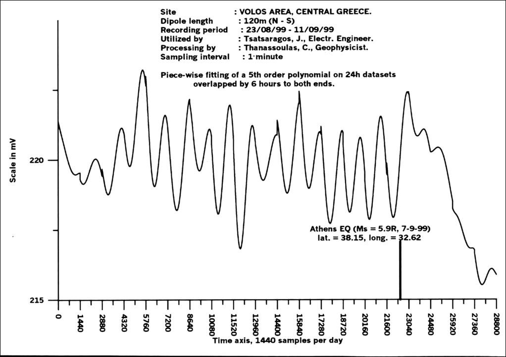
Fig. 3.16.2.1. Earth’s electric oscillatory field recorded by VOL monitoring site, prior to Athens, earthquake (M=5.9R) in Greece (1999).

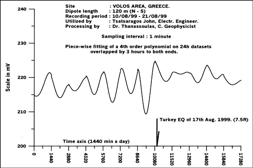
Fig. 3.16.2.2. Earth’s electric oscillatory field, recorded by VOL monitoring site, prior to Izmit, earthquake (M=7.5R) in Turkey (1999).

Fig. 3.16.2.3. Earth’s electric oscillatory field, recorded by ATH monitoring site, prior to South Creta, earthquake (M=5.1R) in Greece (2003).

Fig. 3.16.2.4. Earth’s electric oscillatory field, recorded by PYR monitoring site, prior to Saros Gulf, earthquake (M=5.9R) in Turkey (2003).

Fig. 3.16.2.5. Earth’s electric oscillatory field, recorded by PYR monitoring site, prior to South Creta, earthquake (M=5.1R) in Greece (2003).

Fig. 3.16.2.6. Earth’s electric oscillatory field, recorded in VOL monitoring site, prior to Skyros, earthquake (M=6.1R) in Greece (2001).

Fig. 3.16.2.7. Earth’s electric oscillatory field, recorded by ATH monitoring site, prior to Lefkada, earthquake (M=6.4R) in Greece (2003).

Fig. 3.16.2.8. Earth’s electric oscillatory field, recorded by PYR monitoring site, prior to East Kythira earthquake (M=6.9R) in Greece (2006).

3.16.3. Very Long Period (VLP, plateau-like), seismic, precursory signals have been occasionally recorded, prior to strong earthquakes and indicative samples are presented in the following figures:

Fig. 3.16.3.1. Very long period (VLP) plateau-like, Earth’s electric field (lower graph), recorded by VOL monitoring site, prior to Izmit earthquake (M=7.5R) in Turkey (1999). This plateau-like signal was obtained by applying the “noise injection technique” on the raw data, presented on the upper graph.

Fig. 3.16.3.2. Very long period (VLP) plateau-like Earth’s electric field (lower graph), recorded by VOL monitoring site, prior to Milos, earthquake (M=5.2R) in Greece (2002). The VLP is observed only in the NS component of the Earth’s electric field.

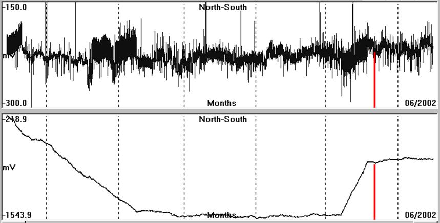
Fig. 3.16.3.3. Original raw data, of the NS component (upper graph) of the previous case, are compared with the resulted data (plateau-like, lower graph), after the application of the “noise injection technique”. Notice the location coincidence of the SES, observed, in the upper graph with the large potential gradients parts of the lower graph.

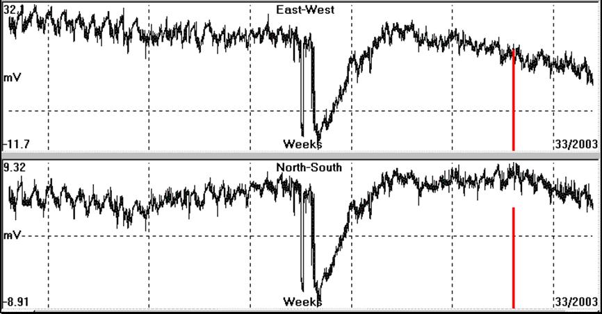
Fig. 3.16.3.4. Very long period (VLP) seismic, precursory, electric signal, recorded by ATH monitoring site, prior to Lefkada earthquake (M=6.4R) in Greece (2003).

Fig. 3.16.3.5. Very long period (VLP) seismic, precursory, electric signal, recorded by PYR monitoring site, prior to East Kythira, earthquake (M=6.9R) in Greece (2006).

   Considering the examples of seismic, precursory, electrical signals, already presented, the following must be pointed out:

   - The referred generating mechanisms, do not justify all types of presented, signals. Actually, only the piezoelectric mechanism explains all kinds of signals, observed, in a satisfa-ctory way.

   - The main difference between the proposed, different mechanisms and the piezoelectric one is that, piezoelectricity is a reversible, large scale, macroscopic mechanism, while the electrokinetic one is not, and the rest of the mechanisms refer to the detailed, stress-load states of the crystalline lattice status of a stress deformed material at a very small scale.

   - The conformity of the electrical precursory signals to the piezoelectric mechanism, combined with the fact that quartz crystals are largely present, as a constituent element of the lithosphere, strongly suggests the use of this phenomenon, as the main, generating mechanism of the seismic, precursory, electrical signals.